1. Introduction
Water is necessary for the survival of all living organisms in the world. Water is life, and demand for it is increasing due to rapid increases in population, urbanization, and industrialization. Moreover, water is a primary need for domestic, industrial, and agricultural activities (Mehta et al. 2022). Thus, it is essential to carefully manage and plan water resources to reduce loss of life and property damage caused by drought, floods, or heat waves (Ali, Shahbaz 2020; Mangukiya et al. 2022). Climate changes influence the hydrological cycle globally; the resulting variations in weather and climate have increased the risks of drought and floods because weather changes, variations in precipitation, peak flows, and extreme temperatures have impacts on river discharge (Mehmood et al. 2021). The amount of discharge generated from a catchment depends on various factors such as duration, meteorological variables, velocity, and water level (Gleason et al. 2014; Saidi et al. 2018; Malik et al. 2020). Therefore, it is necessary to model river discharge using information on the weather at the relevant hydrological station (Dariane, Azimi 2018).
In the past thirty years, stochastic, physical, black box (machine learning and statistical), and conceptual models have been widely applied in hydrological studies. Physical models have been used for hydrological modeling, but their successful application is bound to the complexity of governing equations and the difficulty in measuring the parameters involved (Yousuf et al. 2017). Statistical models try to determine the relationships within the actual data. Their application is limited when data have unique and complex characteristics such as non-linearity, multicollinearity, volatility, irregularities, noise, outliers, and more. In the past two decades, machine learning models have gained importance in hydrology due to their flexibility in handling datasets with unique characteristics (Ravindran et al. 2021; Elbeltagi et al. 2022). Rasouli et al. (2012) applied a support vector machine (SVM), Bayesian neural network, and Gaussian process to predict non-linear river discharge in North America using climate and weather variables. Ali and Shahbaz (2020) applied an artificial neural network (ANN) to predict river discharge in the upper Jhelum River basin of Pakistan.
Although data-driven (statistical and machine learning) models are applied to predict river discharge, there is no single model that can predict river discharge without bias or with utmost certainty (Mehmood et al. 2021). Literature shows that researchers have developed hybrid models by combining two or more techniques to improve the prediction ability of the models (Shabbir et al. 2024). Wang and Li (2018) introduced a hybrid framework based on an error correction approach using the generalized autoregressive conditionally heteroscedastic (GARCH) model when inherent correction and heteroscedasticity of errors cannot be ignored. Zhang et al. (2018a) developed an error-correction-based hybrid framework using an autoregressive (AR) model to predict water levels with improved accuracy. Luo et al. (2019) suggested a hybrid framework based on a composition of factor analysis, decomposition of time series, data regression, and error suppression to predict river discharge. Yan et al. (2020) combined a generalized additive model (GAM) with principal component analysis (PCA) to model the relationship between water level and macroinvertebrate diversity index in the Baiyandian Lake of China. Mehr and Gandomi (2021) suggested a hybrid model by integrating a multi-stage genetic programming (MSGP) model with the least absolute shrinkage and selection operator (LASSO) for improved prediction of river flow. Emadi et al. (2022) modeled river water using a hybrid evolutionary data-driven approach.
River discharge estimation is challenging in hydrological studies because its generation depends on various factors such as rainfall patterns, spatial-temporal irregularities, climatic changes, and many more (Cheng et al. 2019; Hu et al. 2022). In literature, much discussion is on the time series prediction of river discharge (see Luo et al. 2019; Mehr, Gandomi 2021; Adnan et al. 2022). There is an essential need to develop new methods to evaluate the possible influence of different factors on the generation of river discharge. Keeping in view this gap, this study aims to develop a new hybrid approach to examine the relationship between river discharge and meteorological variables.
A new hybrid framework named LAES (LASSO-ANN-EMD-SVM) is proposed in this study based on a combination of feature selection, an ANN model, and an error correction method. In the first stage, LASSO is used to identify meteorological variables that have significant relationships with river discharge. The variables identified by LASSO are then used as input variables to the ANN model to obtain the discharge predictions, and then the error series is computed. Further, the empirical mode decomposition (EMD) technique is used to decompose error series into intrinsic mode functions and residuals. These components are modeled using the SVM model, and their predictions are aggregated. The final discharge prediction is obtained by adding the LASSO-ANN discharge predictions with EMD-SVM error predictions. Application of the proposed LAES hybrid framework is demonstrated for the Kabul River of Pakistan, and its prediction performance is compared with different models.
The proposed hybrid framework is novel as it efficiently predicts river discharge by considering the influence of meteorological variables that have a significant impact on river discharge using LASSO. In addition, the error correction approach in the proposed LAES hybrid model helps to enhance the prediction of discharge by capturing the randomness and volatility of the error series. It provides reliable estimates of river discharge and can be helpful in the management of water supply and flood control.
2. Methods
2.1. Multiple linear regression
The multiple linear regression (MLR) model is a simple and widely used modeling technique. The MLR model is given as:
yj = β0 + β1x1j + β2x2j + … + βpxpj + uj, j = 1,2, . . . , n (1)
where yj is the dependent (output) variable, βj are the regression coefficients, xj are the independent (input) variable, n is the number of observations, p is the number of independent variables, and uj is the residual term.
2.2. Least absolute shrinkage and selection operator
Tibshirani (1996) introduced the least absolute shrinkage and selection operator (LASSO) as a variable-selection approach for regression models. The method minimizes the residual sum of squares subject to the absolute values of the regression coefficients. LASSO performs variable selection and regularization simultaneously to enhance the interpretability and precision of statistical models (Tibshirani 1996). This study applies LASSO to determine important meteorological variables for predicting river discharge.
Assuming a sample contains M events where each event has p number of independent variables and one dependent variable, let yi be the dependent (output) variable, and xi = (x1, x2, … , xp)T be the vector of ith independent (input) variables, then the objective function of LASSO is:
where λ is a pre-determined parameter that determines the regularization degree and β = (β1, β2, … , βp) is the vector of regression coefficients. Let X be the matrix of independent variables, i.e. Xij = (xi)j, where i = 1, 2, … , M, j = 1, 2, … , p and xiT is the ith row of X. Then, the above formula in a compact form can be written as:
where
2.3. Artificial neural network
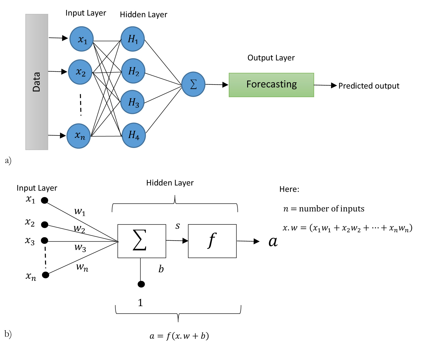
The artificial neural network (ANN) is a robust modeling tool in which information processing is a representation of biological systems (Kachrimanis et al. 2003). The network is constructed from interconnected neurons, which can determine values from the inputs through network processing. The neuron receives input signals and provides the output signal that mainly depends on the neuron processing function. The ANN architecture consists of a series of interlinked neuron layers. Every layer is linked with another layer through neurons, which transfer information between these layers. Through this processing, the information reaches the output (dependent variable) layer. The ANN mechanism follows four assumptions:
Inputs are handled by neurons.
Through the connection of neurons, the information of inputs is passed on to the adjacent layers.
Each neuron has a weight, and the output from the neuron is the product of its input and its associated weight.
The transmitted inputs are passed via the activation of neurons to obtain the output.
Figure 1a shows the architecture of the ANN model, and Figure 1b presents the structure of a neuron where every input (independent variable) comes from other neurons and are multiplied by their weights (wj; j = 1,2, … , n) respectively and then aggregated with the bias (b) vector. This aggregated input (s) is passed using the transfer or activation function (f) to obtain the output (a) of a specific neuron. Letting x be the vector of independent (input) variables, the neural network maps into another output vector a through:
a= f(x. w +b) (4)
The mean squared error (MSE) is computed and using the back-propagation process, the weights of the entire network are modified in the training process. The accuracy of the ANN depends on the quality and amount of data in training.
In this study, the ANN algorithm is trained by a back-propagation technique where the output and input variables are applied in the network. The Broyden-Fletcher-Goldfarb-Shanno (BFGS) optimization is employed in a three-hidden-layer network. In the input layer of the ANN algorithm, the activation function is applied with 1000 iterations in the hidden layers. In this study, the ANN algorithm is applied using the validant library in the R programming language.
2.4. Empirical mode decomposition
Huang et al. (1998) introduced empirical mode decomposition (EMD) as an adaptive method for signal analysis. The EMD is designed to analyze non-linear series. The EMD approach assumes that a signal contains different intrinsic mode functions (IMFs) of oscillations. Every mode has the same number of extrema and zero-crossings. There is a single extremum between successive zero-crossings. In this way, the signal is decomposed into different IMFs and residuals. A component is an IMF if it satisfies two conditions: (i) the number of extrema and the number of zero-crossings must be equal to one or differ at most by one, and (ii) at any point, the average of the envelope is zero (Huang et al. 1998). Any original signal y(t) can be decomposed using the EMD algorithm as follows (Lei et al. 2003; Jungsheng et al. 2006):
a) Find the local minima and maximum through the cubic spline line as the upper envelope and lower envelope, respectively.
b) Find the mean (m1) of upper and lower envelopes.
c) The difference between the y(t) and the 1st component m1 is the first component denoted as h1 i.e. h1 = y(t) − m1. If h1 is an IMF, then it is said to be the first IMF component of y(t).
d) If h1 is not an IMF, then it is treated as an original signal, and the steps (a)-(c) are repeated, then h1 − m11 = h11.
After repeating the sifting process k times, h1k becomes an IMF, i.e. h1(k−1) − m1k = h1k, then it is termed as:
c1 = h1k (5)
The first IMF component from the data.
e) Next, subtract c1 from y(t) to obtain u1 = y(t) − c1 where u1 denotes the treated data, and the process is repeated n times to get n IMFs of y(t). Then,
At the end of the process, we have IMFs (cj; j = 1,2, … , n) and residual (uj). By summation of all the components, the original signal y(t) can be obtained as:
The EMD method is implemented using the EMD library in R language in this study.
2.5. Support vector machine
Support vector machine (SVM) is a popular modeling technique for classification and regression problems. The SVM algorithm maps complex high-dimensional data into high-feature space (Vapnik 1995). We assume a training set with n observations, {xd, yd}, d = 1,2, … , n, xd ε R, yd ε R, where yd denotes the estimated value of the dependent (output) variable, xd is the corresponding lagged values of the dependent variable, and n is the sample size. Then, the SVM is developed as:
f(x) =ωTφ(x) + b (8)
where f(x) is the estimated dependent variable, b ∈ R is the bias, and ω ∈ R represents the vector of weights. The transfer function φ(x) maps input data into high-dimensional space. The Eq. (8) is solved by risk minimization as follows:
where c > 0 represents the penalty parameter, ξ and ξ* are slack variables that show the upper and lower constraint of f(x), and ε denotes the insensitive loss function. Further, the Lagrangian function is used as the non-linear regression function, which replaces φ(x) and ω in Eq. (8) as:
where k(x, xd) = ⟨φ(x), φ(xd)⟩ is the kernel function. The αd* and αd represents the Lagrange coefficients.
In this study, SVM is applied to capture the features of the error series using the radial basis function (RBF) kernel, i.e. k(x, xd) =
3. Proposed hybrid framework
In this paper, we propose a novel LASSO-ANN-EMD-SVM (LAES) hybrid framework to predict daily river discharge based on its relationship with the meteorological variables. The proposed LAES hybrid framework is displayed in Figure 2.
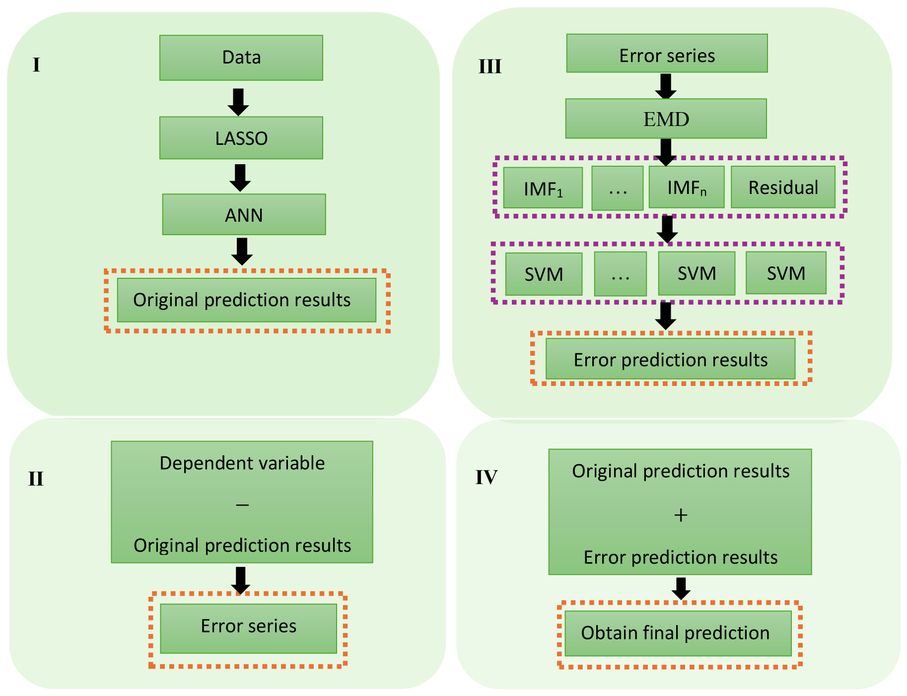
The steps of the LAES framework are:
LASSO is applied for the selection of meteorological variables that influence discharge (y) of the river.
Next, the ANN model is employed to model river discharge using meteorological variables as independent variables and the predictions of river discharge (ŷLA) are obtained. Further, the error (i.e. ê = y − ŷLA) is computed.
Using EMD, the error is decomposed into sub-series, and then the SVM model is used to predict each sub-series. By aggregating them, the predicted error (êES) is obtained.
The final river discharge prediction is obtained using the predicted error series to correct the predicted river discharge in stage II (i.e. ŷLAES = ŷLA + êES).
The proposed LAES hybrid method is a unique combination of the feature selection method with the ANN model and error correction approach. To the best of our knowledge, there is no hybrid model in the literature that integrates LASSO with an error correction approach for modeling non-linear and high-dimensional data sets.
3.1. Limitations of LAES hybrid framework
The efficiency of the LAES hybrid framework depends on the optimal choice of parameters of the LASSO approach. This framework works efficiently when the independent variables are selected using the optimal value of the LASSO parameter and the information loss by dropping variables is minimal. A high value of the LASSO parameter can contribute toward a loss of information, which may result in poor model fit. Secondly, the performance of the proposed hybrid method depends on the availability of data variables that may vary in different regions of the world due to differences in weather characteristics. The performance of the LAES hybrid model may vary with respect to changes in region (or location) of study and climatic conditions.
4. Application
Data and performance measures are described in this section. The codes of this study were written in R language version 4.1.0. The complete analysis is performed on a personal computer with an Intel Core i9-9900 CPU (32GB RAM).
4.1. Description of data
The Khyber Pakhtunkhwa province is a mountainous region, including the Tirich Mir, Lalazar, Hindu Kush, and some other mountain ranges. The changing climate of this region affects air temperature, water flows, precipitation, and groundwater resources for irrigation systems and domestic use. These conditions make the northern area of Pakistan prone to drought or flooding due to changing environment and weather conditions.
The Kabul River begins at the Unai pass base from the Hindu Kush mountains in Afghanistan, flowing toward the east and spanning 700 km to drain into the Indus River of Pakistan (Mehmood et al. 2021). The Kabul River at Nowshera station is located at a latitude of 34°0'25''N and longitude of 71°58'50''E. The hydrometeorological regime is characterized by rain in the spring and snow in the winter. The melting of glaciers in summer is increasing each year due to high temperatures, leading to rising water levels in the river (Rasouli 2022). In addition, rainfall in the monsoon season also affects water levels in the river. The Kabul River is influenced by varying climatic conditions, which may lead to hydrometeorological hazards (i.e., heatwaves, floods or drought).
Figure 3 shows the location of the Kabul River in Pakistan. Kabul River data was collected from the Surface Water Hydrology Project (SWHP) Department of the Water and Power Development Authority of Pakistan (WAPDA) from 1st January 2005 to 31st December 2017. The data contain river discharge and meteorological variables. The meteorological variables include air temperature (minimum and maximum), pan water (minimum and maximum), relative humidity (8 AM and 5 PM), dew point (8 AM and 5 PM), evapotranspiration, and wind speed. Average temperature and precipitation have high variability across the basin. River flow has been high during the monsoon period in Pakistan, particularly in July and August. In the midst of 2005, 2010, and 2015, there was extensive flooding due to high temperatures and heavy rainfall in the region. The discharge had some missing values, which were replaced with the monthly average (mean) value. Outliers present in the data were also replaced by median of the respective month. The number of observations for each variable is 4748, approximately 365 daily values for 13 years.
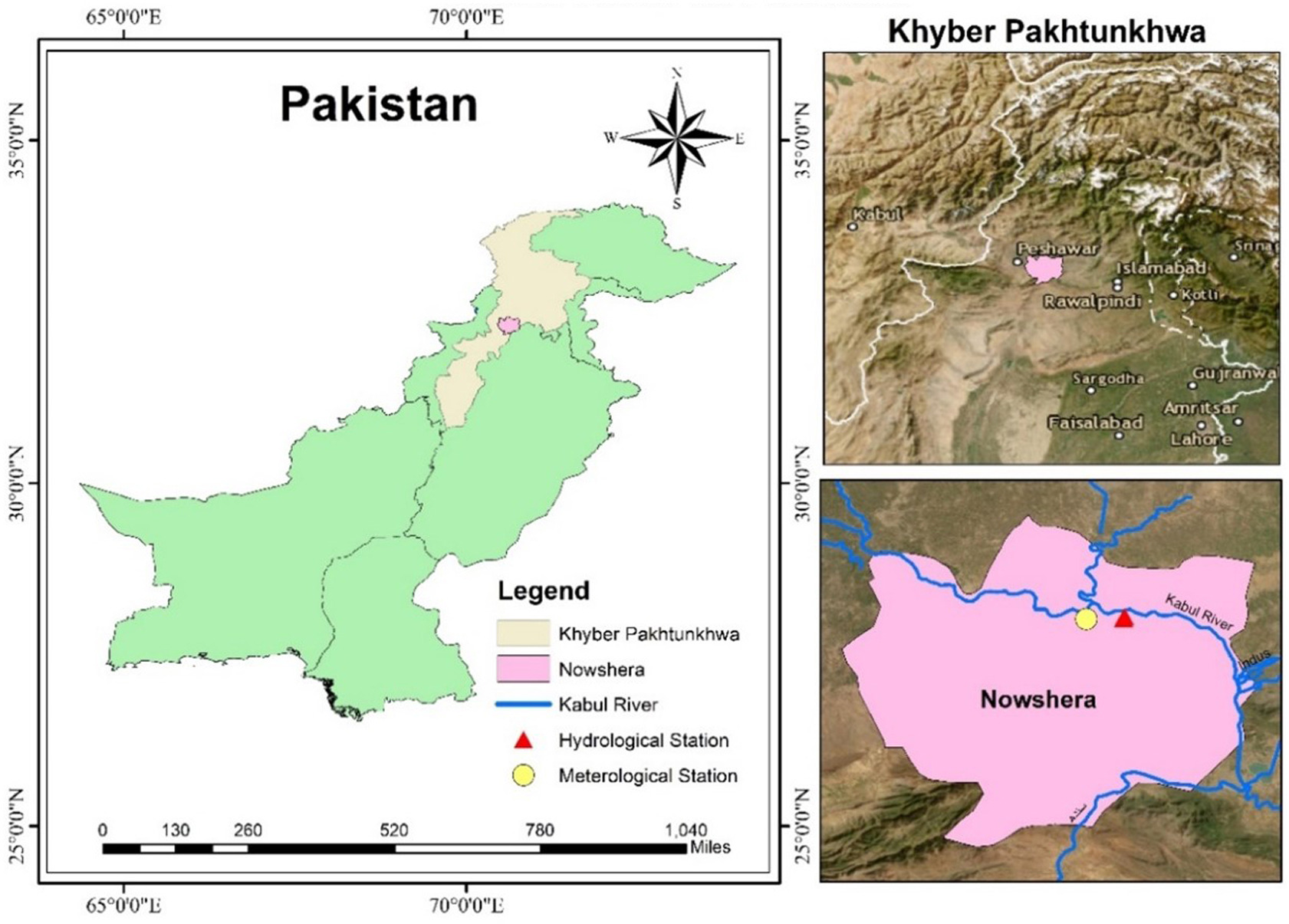
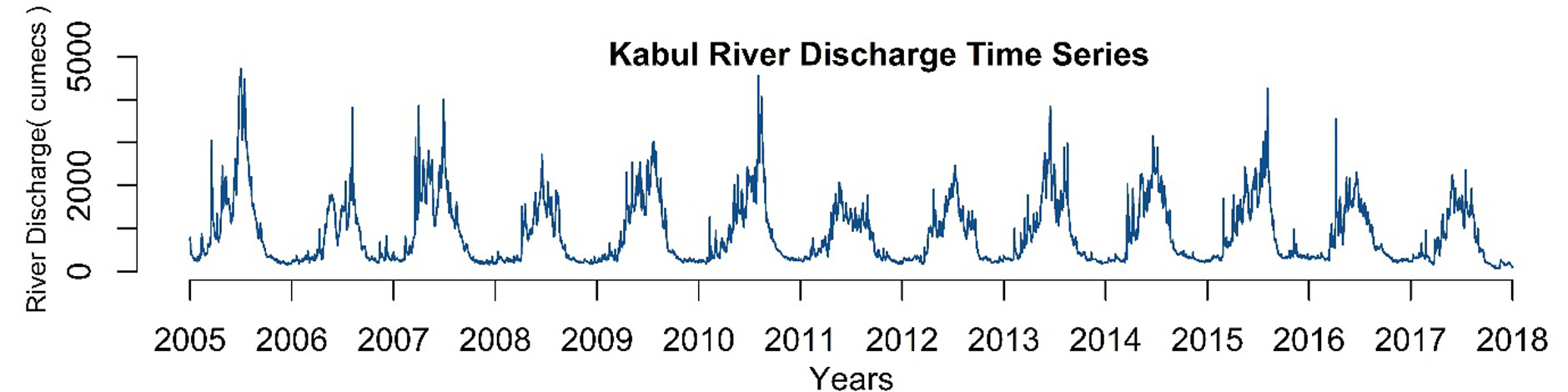
Table 1 shows summary descriptions of all the variables of the Kabul River data. The air temperature (maximum), air temperature (minimum), pan water (maximum), pan water (minimum), dew point (8 AM and 5 PM), relative humidity (8 AM and 5 PM) have negatively skewed distributions, while river discharge, wind speed, evapotranspiration, precipitation and rainfall have positively skewed distributions. The average discharge in the Kabul River is 871.8 m 3/s. Figure 4 shows the Kabul River discharge series. It shows that there are non-linear relationships between river discharge and all meteorological variables.
Table 1.
Descriptive summary of variables.
The data variables were normalized using the following (Duan et al. 2021):
where z is the original data variable, znormal is the normalized data variable, zmin is the minimum value, and zmax is the maximum value of the original data variable. After normalization, the dataset is divided into two parts, where 80% of the data are used for training and the remaining 20% for testing (Kisi et al. 2021; Shabbir et al. 2022). The performance of models is evaluated by 5-fold cross-validation using different performance evaluation measures and the average results of these indicators for training and testing data.
4.2. Performance evaluation measures
The prediction performance of the proposed hybrid framework is evaluated on both training and testing datasets. A 5-fold cross-validation approach and different goodness-of-fit measures are selected to assess the performance of models. These measures include root mean square error (RMSE), mean absolute percentage error (MAPE), root-relative square error (RRSE), mean absolute error (MAE) and coefficient of determination (R 2). These measures are given as follows (Zeinali et al. 2020; Shabbir et al. 2023):
where n denotes the total number of observations, yj denotes the actual observation and ŷj denotes the predicted values. The terms ȳ and
To compare the performance of the different models for river discharge prediction, the improvement percentages of RMSE, MAPE, RRSE, and MAE are also used and are given as:
where subscript i denotes the competing model and subscript j indicates the proposed LAES hybrid model. These quantities indicate the degree of improvement in the prediction performance of one model relative to another model (Duan et al. 2021).
The Diebold-Mariano (DM) test has been widely used in literature to compare the forecast accuracy of two models (Silva et al. 2021; Shabbir et al. 2022). The null and alternative hypotheses are:
H0: E[dt] ≥ 0 (22)
H1: E[dt] < 0
where dt is the difference loss function, i.e., dt = e1t − e2t, e1t and e2t denotes the set of prediction errors of two competing models. The test statistic is
In this study, a one-sided DM test is used to compare the prediction accuracy of the LAES model with six models. This test uses subscript 1 for the proposed LAES model and subscript 2 for the competing models. This test is applied using the squared differences loss function to compare models at a 1% significance level. If DM < −2.326, we will reject the null hypothesis. The proposed LAES hybrid model is compared with MLR, SVM, ANN, LASSO-MLR, LASSO-SVM and LASSO-ANN models in this study.
5. Results and discussion
In the proposed hybrid framework, LASSO is employed to choose meteorological variables that have significant roles in predicting Kabul River discharge. This step eliminates insignificant variables and constructs a better prediction model. Using LASSO, we retain only important input variables that influence the river discharge of the Kabul River. The results of the LASSO using λ = 0.010 are shown in Figure 5a. LASSO eliminates three meteorological variables, i.e., pan water (maximum), relative humidity (8 AM) and relative humidity (5 PM). The air temperature (minimum and maximum), dew point (8 AM), relative humidity (5 PM), rainfall, precipitation, wind speed, and evapotranspiration are significant variables for prediction of river discharge. These variables. {x1, x2, x4, x5, x8, x9, x10, x11, x12} are used as inputs to LASSO-based models. Bui et al. (2019) stated that dew point is a component of the temperature variable. The precipitation and rainfall factors are dependent on the air temperature and are indirectly associated with the dew point.
Fig. 5.
The variable screening (a) and variable importance (b) results from LASSO on Kabul River data.
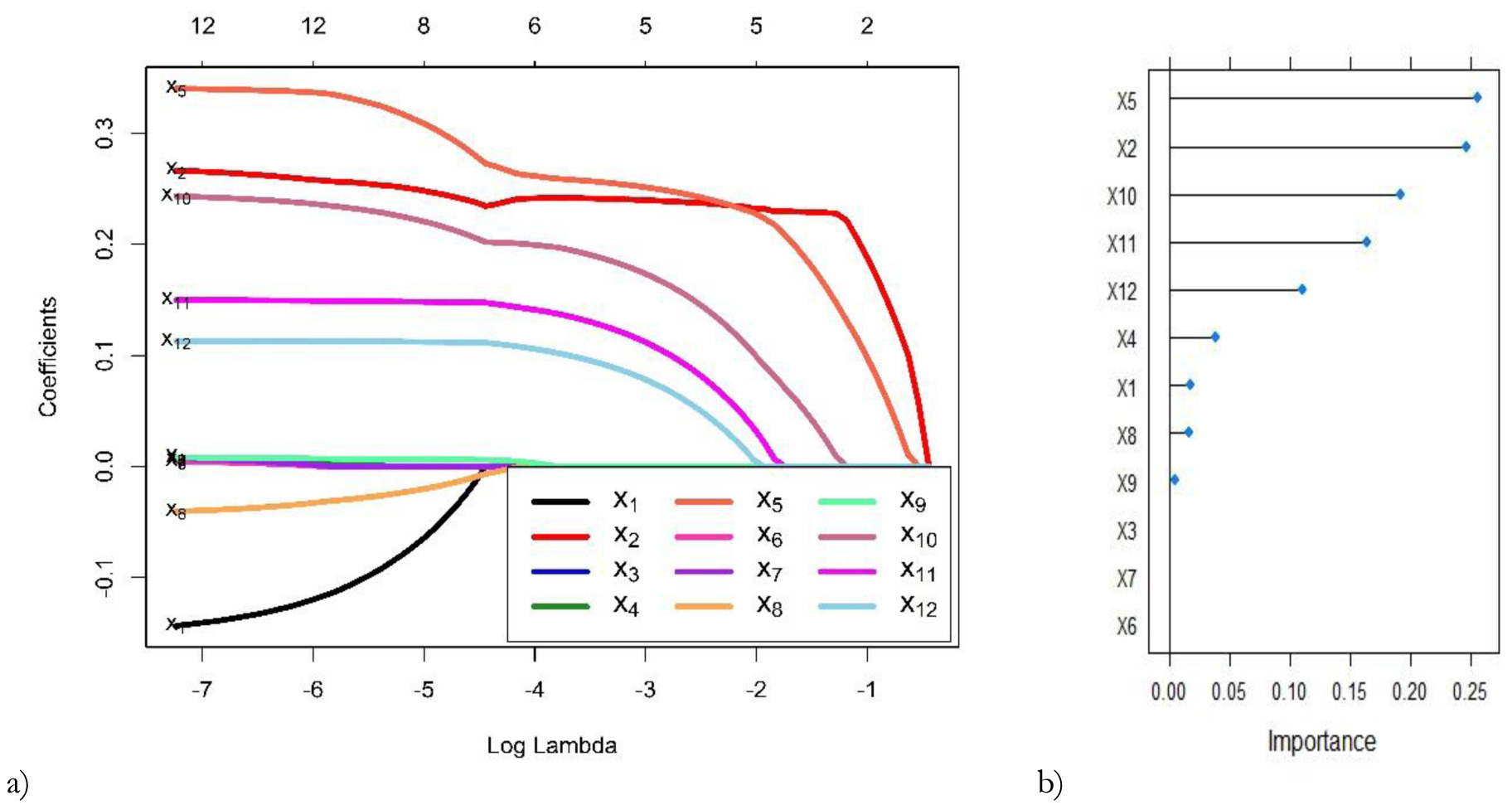
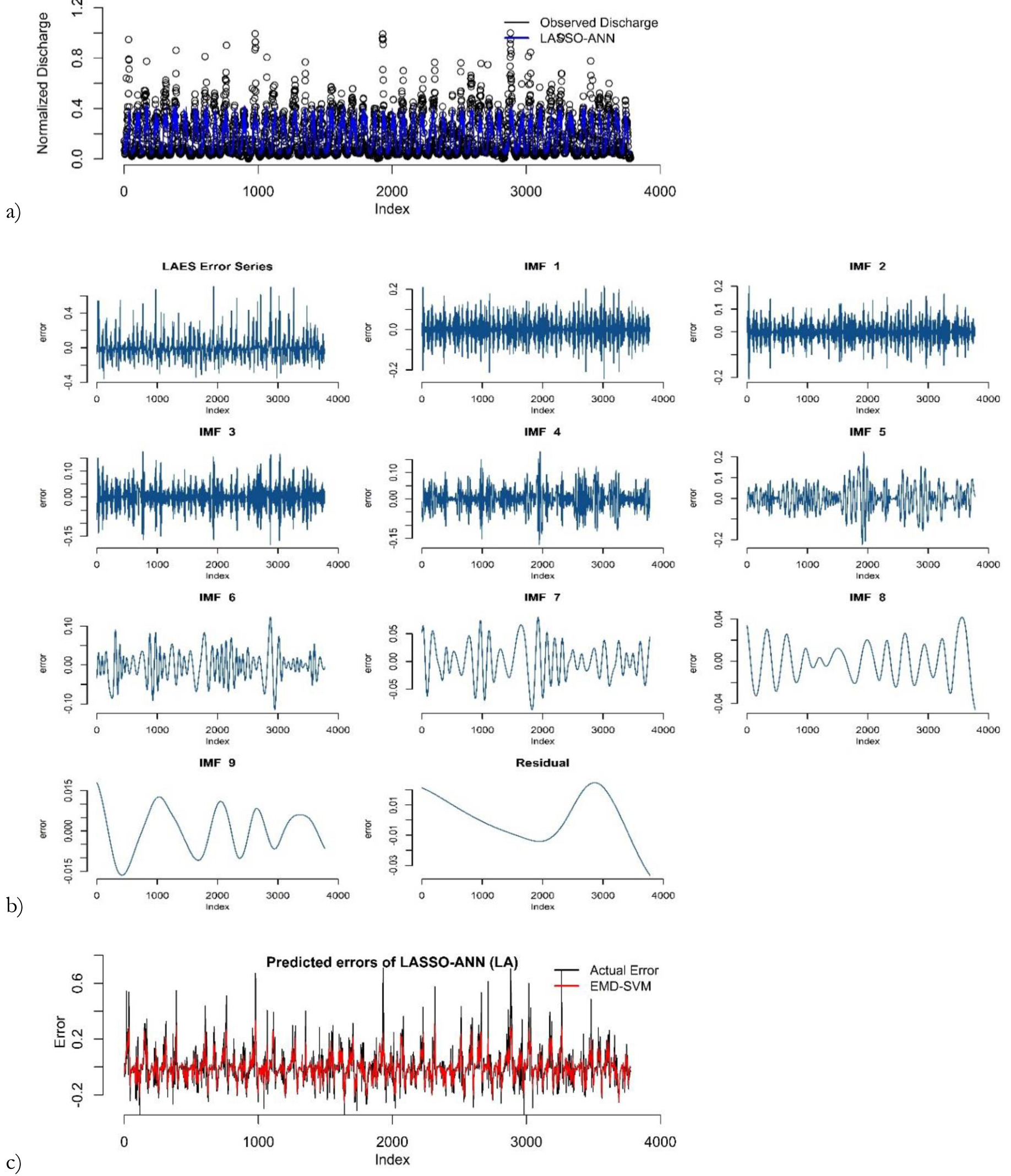
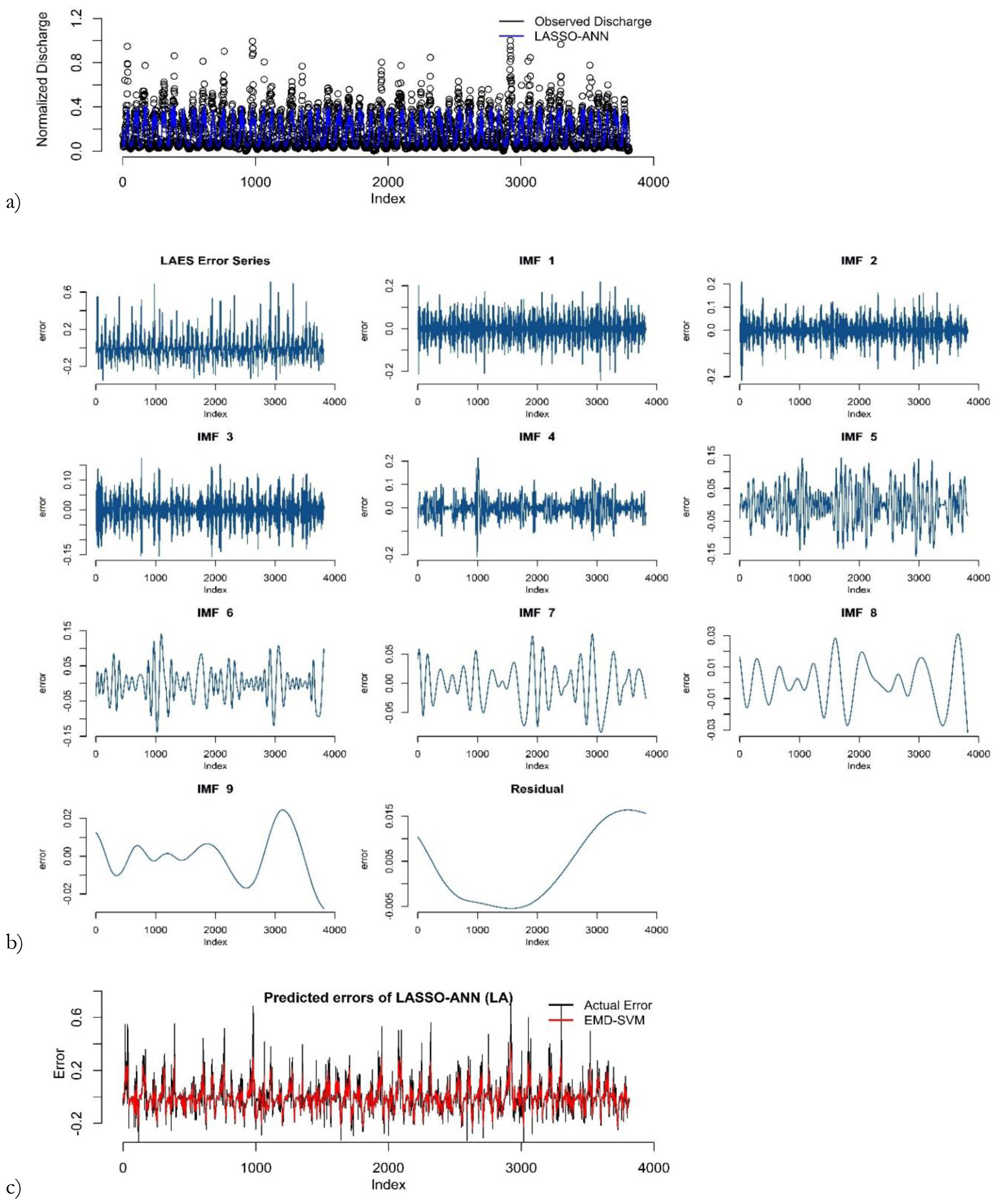
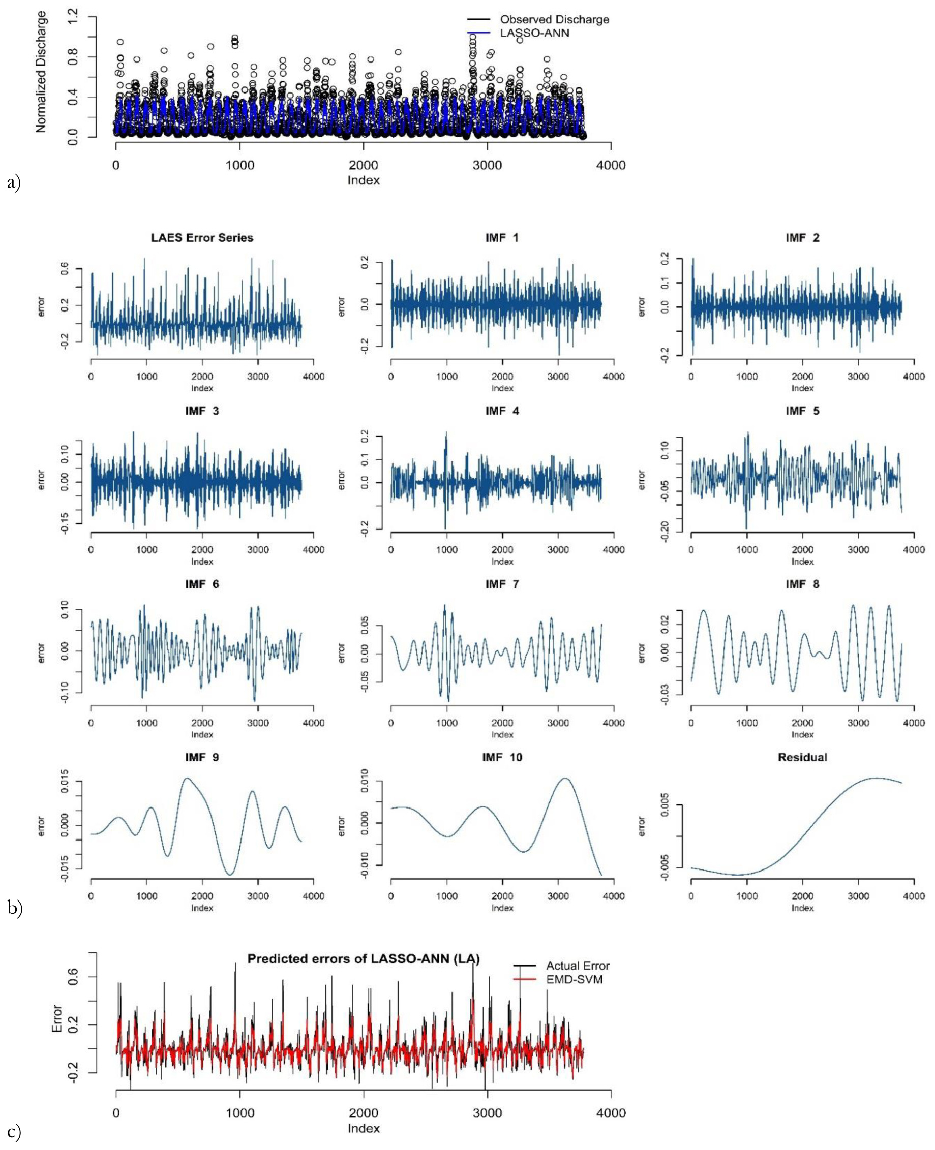
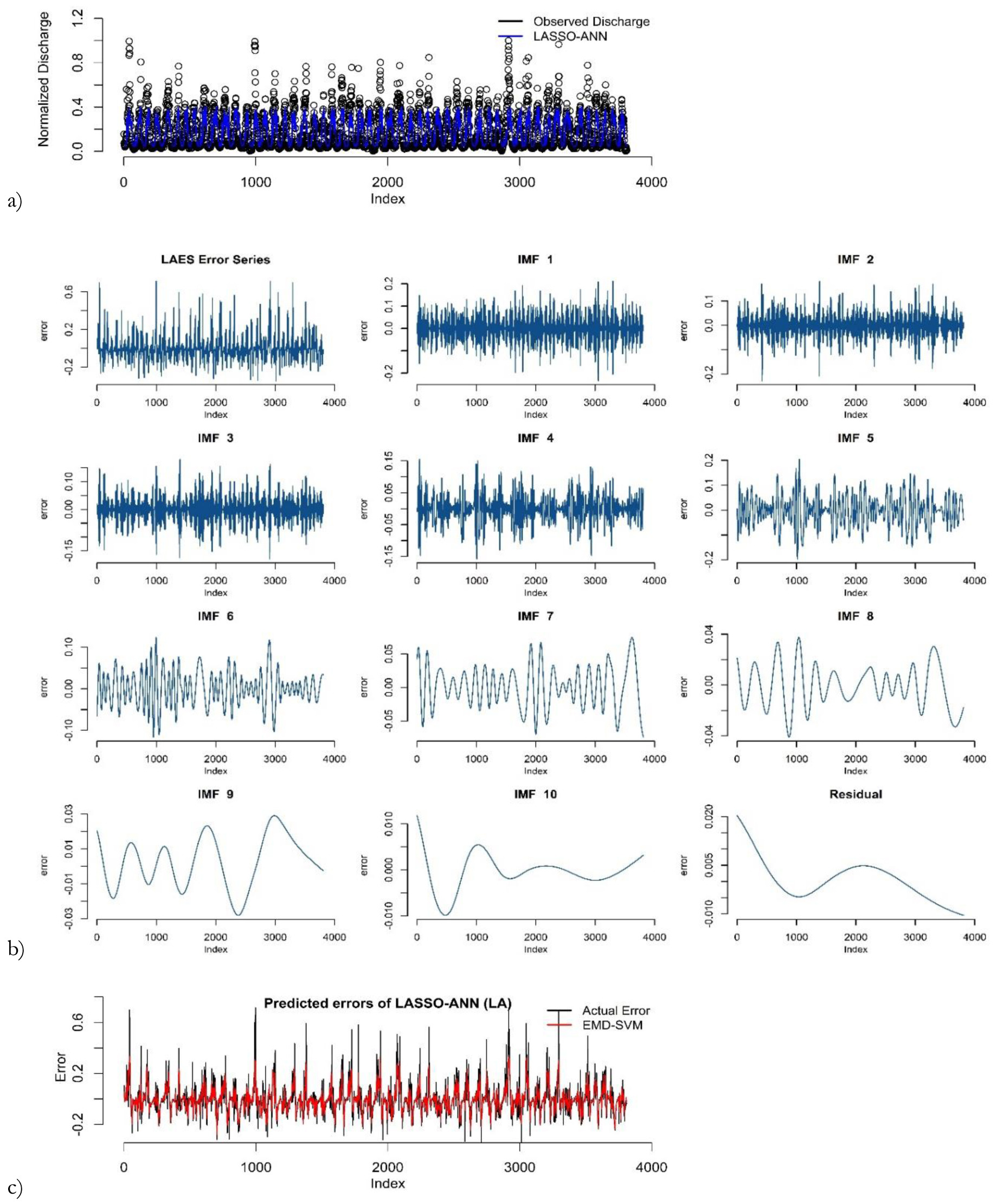
Figure 5b shows that dew point (8 AM) is the most significant variable for predicting river discharge. These variables selected by LASSO are used as inputs to the ANN model in the proposed hybrid framework. The prediction results by LASSO-ANN in the first round of the training phase are demonstrated in Figure 6a. The results of the remaining rounds are given in supplementary materials.
Fig. 6.
Prediction results of LASSO-ANN: (a) error decomposition using EMD; (b) modeling of decomposed components (c) in the first round of training the phase for the Kabul River.
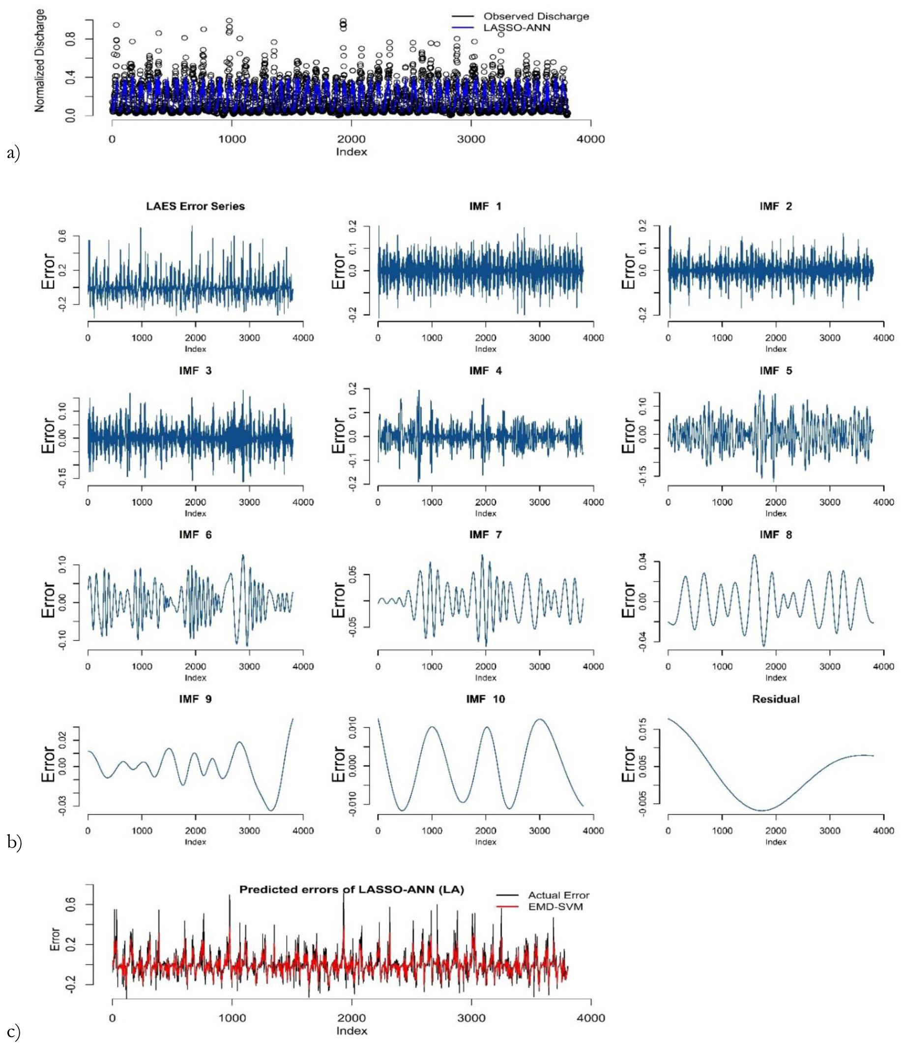
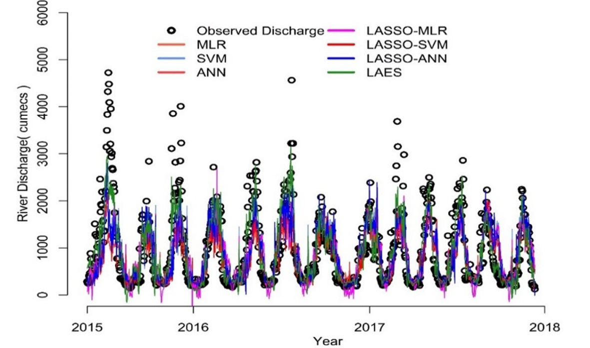
After ANN model training, the predictions and error series are obtained. Stationarity of the error series is checked using an augmented Duckey-Fuller (ADF) test. The Dickey-Fuller statistic is –3.3875, indicating that the error series in the first round is non-stationary at the 5% level of significance. The results of ADF tests of the remaining rounds are provided in the supplementary materials. Next, the EMD decomposes the error series into IMFs and residuals as shown in Figure 6b. Then, the SVM is applied to model each component of the decomposed error series. The sub-series predictions are obtained and aggregated as the final error prediction shown in Figure 6c. The final prediction of river discharge is computed by adding the predicted errors and predicted river discharge. Lastly, the actual predicted values of river discharge are obtained by anti-normalization using Eq. 11. Figure 7 shows the predicted discharge plot in the testing phase in the first round. It reveals that the proposed LAES hybrid models have the closest predictions to the observed river discharge.
5.1. Comparison of model accuracy
The daily river discharge was estimated against various meteorological variables. Table 2 presents the training and testing phase results of daily river discharge prediction. In the training phase, the MLR model is the worst performer among all models (RMSE = 533.822 m 3/s, MAE = 378.003 m 3/s, RRSE = 0.711, MAPE = 66.786% and R2 = 49.4%). However, the SVM and ANN models performed relatively better than the MLR model. For example, in the training phase, the RMSE for MLR, SVM and ANN models is 533.822 m 3/s, 511.262 m 3/s and 507.015 m 3/s, respectively. Similar to this study, Zhang et al. (2018b) found that the MLR model is the worst performer for predicting river discharge in the East River basin of China. Some other studies found that the non-linear features of river discharge are captured well by SVM and ANN models (see Poul et al. 2019 and Meng et al. 2021).
Table 2.
Performance analysis of the proposed model with different models.
Comparing the performance of models based on meteorological variables selected by LASSO, we found that the performance of all models is improved in most of the instances. The performance of the LASSO-MLR model is better than the MLR model in the testing phase (RMSE = 543.559 m 3/s, MAE = 381.889 m3/s, RRSE = 0.725, MAPE = 67.758% and R2 = 47.4%). However contrary results are obtained in the training phase, in which the LASSO-MLR model has a similar fit to the MLR model. The prediction ability of LASSO-ANN and LASSO-SVM is better than ANN and SVM models respectively. Mehr and Gandomi (2021) found that LASSO improved the predictive ability of a multi-stage genetic programming model by reducing the number of genes for predicting river discharge in the Sedre River of Turkey. In the training phase, the proposed LAES hybrid model has the best fit for river discharge data based on various performance criteria (RMSE = 302.952 m 3/s, MAE = 201.022 m 3/s, RRSE = 0.404, MAPE = 30.494% and R2 = 83.7%).
Comparing the results in the testing phase, the MLR model has the poorest performance when all the meteorological variables were used as inputs (RMSE = 554.277 m 3/s, MAE = 383.541 m 3/s, RRSE = 0.739, MAPE = 68.134% and R2 = 45.3%). The use of LASSO for dimension reduction enhanced the performance of MLR, SVM, and ANN models in the testing phase. Judging by RMSE, RRSE and R 2, the LASSO-ANN model is a better performer than the LASSO-SVM and LASSO-MLR models. However, comparing MAE and MAPE, the LASSO-SVM model performs better than the LASSO-MLR and LASSO-ANN hybrid models (MAE = 307.124 m 3/s and MAPE = 39.394%). The proposed LAES model outperforms all competing models in the testing phase (i.e., RMSE = 337.143 m 3/s, MAE = 218.353 m 3/s, RRSE = 0.449, MAPE = 32.354% and R2 = 79.8%). Overall, the proposed LAES hybrid model has higher prediction accuracy than single and LASSO-based ANN, SVM, and MLR models.
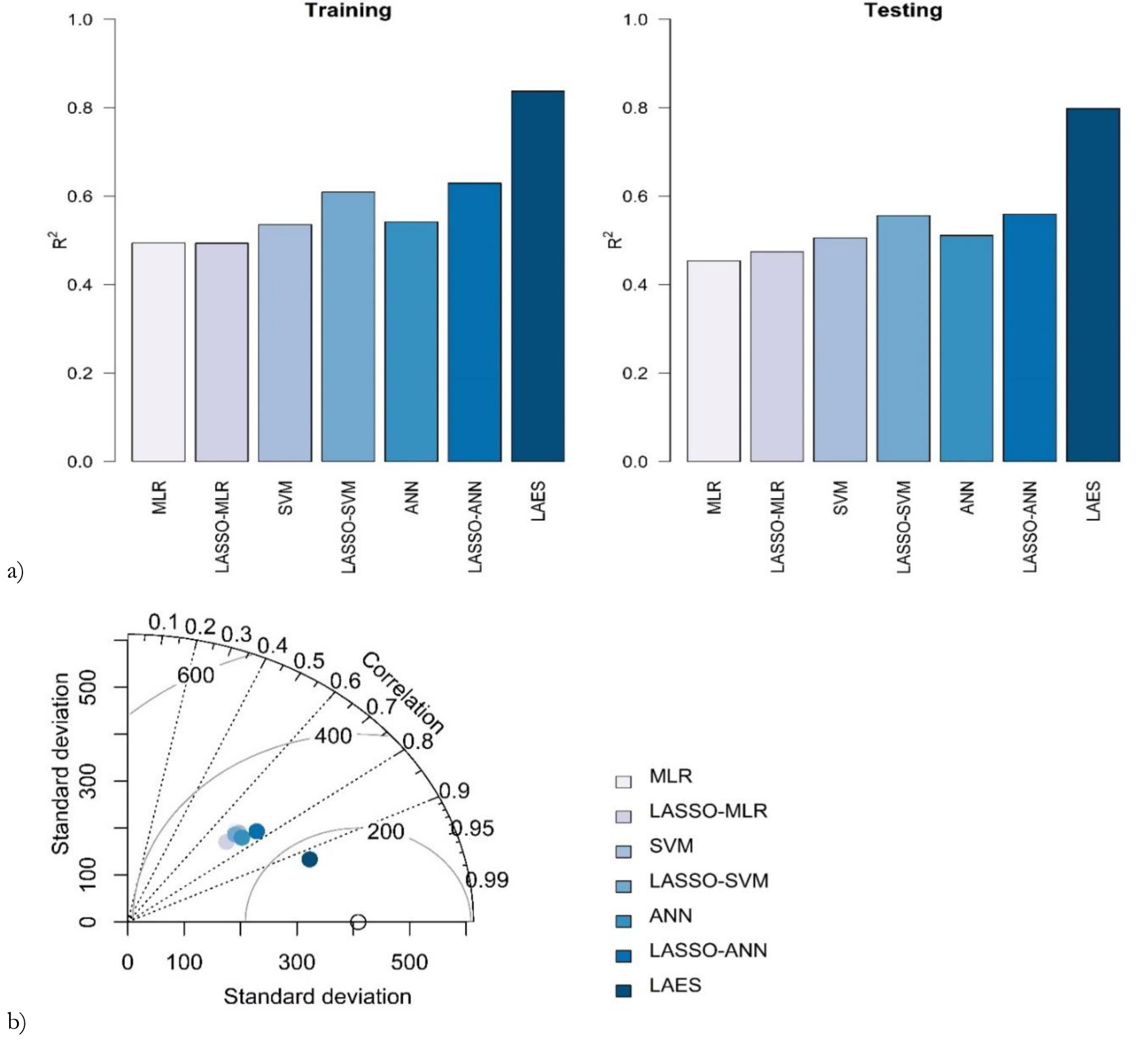
Figure 8a presents the goodness-of-fit measure values of all the models considered in the study in both training and testing data. It shows that the proposed LAES hybrid model has the highest accuracy among all models considered in the study. The Taylor diagram in Figure 8b shows that the proposed LAES model is the most efficient among all models considered in predicting daily river discharge based on its relationship with meteorological variables.
Fig. 8.
Prediction results of models in training and testing phase (a) and Taylor diagram (b) for the Kabul River.
The improvements of the proposed LAES hybrid model are shown in Table 3 in terms of PRMSE, PMAE, PRRSE, PMAPE and PR2 for both training and testing phases. The proposed LAES hybrid model has 43.3%, 40.7% and 40.3% lower RMSE than the MLR, SVM, and ANN models, respectively, in the training phase. The findings indicate that the MLR model is least efficient for non-linear data, consistent with the findings of Zhang et al. (2018b).
Table 3.
Improved percentage (%) of proposed model versus other models.
Comparing the LAES model to LASSO-based models, we found that their promoting improvements were lower compared to single MLR, SVM, and ANN models in the majority of the scenarios. During testing, the reduction in RMSE by LASSO-MLR and MLR models is 38% and 39.2%, respectively. Similarly, the improvements by the LAES model vs. the SVM model (36.1%) are higher than the LAES model vs. the SVM model (32.6%). The proposed LAES hybrid model has 68.2%, 43.6%, and 42.7% better prediction accuracy than the LASSO-MLR, LASSO-SVM, and LASSO-ANN models. Kang et al. (2023) also stated that LASSO helps enhance the predictive performance of monthly run-off, which is influenced by meteorological events.
Generally, the proposed LAES hybrid model has promising predictions compared to all six models. During the training phase, the MAE of LAES compared to MLR, SVM, ANN, LASSO-MLR, LASSO-SVM, and LASSO-ANN decreased by 46.8%, 35.1%, 39.9%, 46.9%, 28.4%, and 33.6% respectively. These results are in agreement with the findings of Duan et al. (2021). They reported that the decomposition-based error correction approach significantly improves the accuracy of models.
The DM test results on the testing data of Kabul River discharge are given in Table 4. The null hypothesis for all competing models is rejected at a 1% significance level. Thus, the prediction accuracy of the proposed hybrid LAES model is higher than the six benchmark models. Therefore, the DM test confirms that the proposed LAES hybrid model has higher prediction accuracy than the competing models in predicting river discharge.
6. Conclusion
In this study, a new hybrid framework named LAES (LASSO-ANN-EMD-SVM) is introduced for modeling river discharge using information from several meteorological variables. The proposed hybrid model is a composite of a variable selection approach with an artificial neural network and error correction method. The application of the LAES hybrid framework is illustrated using the data from the Kabul River in Pakistan. The effectiveness and predictive ability of the proposed framework are compared with six models using different performance measures. The numerical findings reveal that the LAES hybrid model has better prediction performance than the single and LASSO-based MLR, SVM, and ANN models. Judging by RRSE, the LAES hybrid model has 43.3%, 40.8%, 40.3%, 43.3%, 35.5%, and 33.7% lower prediction errors than MLR, SVM, ANN, LASSO-MLR, LASSO-SVM and LASSO-ANN models respectively. The Diebold-Mariano test shows that the proposed LAES model has higher prediction accuracy than all competing models in the study. The proposed LAES model can serve as a successful tool for river discharge prediction by considering the impact of meteorological variables. In this study, we have used the LAES hybrid model for regression modeling only, but it can be applied for time series prediction of hydrological variables (such as river inflow and monthly run-off). For future research, new hybrid models can be developed by considering (i) relevance vector machine (RVM) or deep learning models such as multilayer perceptron (MLP) in modeling; and (iii) using decomposition techniques such as ensemble EMD, complete EEMD (CEEMD), and variational mode decomposition (VMD) methods in the error correction stage. The proposed LAES model can serve as a successful tool for river discharge prediction of catchment areas of different areas of the world for efficient planning of water resources.