1. Introduction
Flood routing is a mechanism to ascertain the timing and magnitude of flow at a point on a watershed from known or assumed hydrographs at one or more points upstream (Fread 1981; Tewolde, Smithers 2006). Hydraulic structures are constructed across the rivers to prevent flood damage. To ensure ample protection from floods and to obtain viable solutions to flooding, we required flood routing. Flood routing helps in designing a proper hydraulic structure for flood control (Barati 2010). Two main approaches, one based on hydrologic routing and the other based on hydraulic routing, are typically used to guide flood waves to natural channels. The hydrological method is based on the equation of storage continuity, while the hydraulic method is based on the equations of continuity and momentum consisting of the Saint-Venant equations (Choudhury et al. 2002; Barati 2010). The outflow hydrograph at the downstream location can be estimated using a flood routing model by routing a flood event from an upstream gauging station, but in developing countries, most of the basins are ungauged.
Various simplified routing models were created in the 20th century. Most of these models have been successfully applied to rivers and reservoirs (Hashmi 1993). Due to the adequacy and reliable relationship between their parameters and channel properties, the Muskingum method (McCarthy 1938) and the Muskingum-Cunge method (Cunge 1969) are widely adopted and used in flood routing models (Fread 1983; Haktanir, Ozmen 1997). The Muskingum model investigates a method of parameter estimation to determine the weight coefficient X and wave travel time K. Yoo et al. (2017) proposed a methodology to determine the Muskingum parameters, using the basin characteristics which represents the inlet and outlet of the channel reach. Most of the methods are optimization techniques, including trial and error, recession analysis (Yoon, Padmanabhan 1993), least-squares (Al-Humoud, Esen 2006), feasible sequential quadratic programming (Kshirsagar et al. 1995), chance-constrained optimization (Das 2004, 2007), genetic algorithm (Chen, Yang 2007), particle swarm optimization (Chu, Chang 2009), harmony search (Kim et al. 2001), Broyden-Fletcher-Goldfarb-Shanno technique (Geem 2006), immune clonal selection algorithm (Luo, Xie 2010), and hybrid algorithm (Lu et al. 2007; Yang, Li 2008). However, because they need large amounts of observed data, these studies and methods are more applicable to flood routing in gauged basins.
It is difficult to predict flow characteristics in ungauged basins (Sivapalan et al. 2003), because streamflow time series are usually not long enough for parameter calibration. Two common ways to address this problem are: (a) the use of physically-based models, and (b) regionalization of model parameters according to the physical characteristics of basins (Yadav et al. 2007). To improve the prediction accuracy of streamflow in an ungauged basin, several regionalization models have been developed, including parametric regression, the nearest neighbor method, and the method of hydrological similarity (Li et al. 2010). Physically-based models are strongly linked to the basin's observed physical characteristics. Many physically based distributed hydrological models have been created and used in ungauged basins to simulate and predict runoff hydrographs. However, differences in scale, over-parameterization, and model structural error remain impediments, and some calibration criteria are generally required. Bharali and Misra (2020a-b, 2021) proposed hydraulic routing methods to estimate the flood hydrograph at the outlet of the ungauged basin. For flood routing models used in ungauged basins, the relationships between physical characteristics and model parameters of gauged basins are useful (Tewolde, Smithers 2006). Consequently, the modification and interpretation of the Muskingum model's parameters in terms of physical properties extends the model's applicability to ungauged basins, as observed by Kundzewicz and Strupczewski (1982).
The Muskingum method is one of the most popular and commonly used hydrologic methods for flood routing. McCarthy introduced it in 1938 for management of the Muskingum River basin in Ohio by the Army Corps of Engineers (Chow 1959; Henderson 1966; Roberson et al. 1988; Li et al. 2019). The original formulation of the method was strictly empirical, with two coefficients that worked together to control translation and attenuation. Initially, it was recognized that one of the coefficients, often referred to as X, was associated with the weight factor, which had the most significant impact on attenuation, whereas the second coefficient, often referred to as K, was related to the time of travel or the translation of the wave through the channel. The X coefficient was limited to the range 0 to 0.5, and to estimate it from calibration data, graphical techniques were developed (Roberson et al. 1988; Fenton 2019).
Long-term discharge observations are usually not available at the appropriate location, and, for various reasons, these records often contain missing data. As a result, many hydrological models have been developed to obtain runoff from rainfall due to the easy availability of rainfall data for longer periods at various locations (Singh, McCann 1980; Singh, Frevert 2005). The Soil Conservation Service Curve Number (SCS-CN) model has been widely used to calculate surface runoff. A theoretical framework for validating the SCS method has been provided (Yu 1998). Yu (2012) showed that the proportionality in the SCS equation would follow retention and runoff if the temporal distribution of rainfall intensity and spatial distribution of the highest infiltration rate were independent and illustrated by an exponential probability distribution. In particular, 'Yu' demonstrated that the highest retention S could be seen as the product of the highest average infiltration rate and effective rainfall duration. Changes were made to the original SCS-CN method by replacing (P – Ia) with 0.5*(P – Ia) (Mishra, Singh 1999). They made comparisons between the current SCS-CN system and the proposed modification, and the new version was found to be more reliable than the existing version. The flood prediction was carried out using the curve number method in the geographical information system (GIS) at the North Karun River field (Akhondi 2001).
The current SCS-CN method was modified and named the MS model by Mishra et al. (2004); the proposed model was based on the SCS-CN method and also incorporated the antecedent moisture while calculating the direct surface runoff. The modified version was evaluated and compared with the existing SCS-CN method, with the observation that the modified MS model's performance was much better than the existing SCS-CN model. In 2005, by considering a large set of rainfall-run-off events, they used the MS model with its eight variants in the field and revealed that the performance of the current version of the SCS-CN method was remarkably poor compared to all model variants. To increase the applicability of the model for complex watersheds with high temporal and spatial variability of soil and land use, some researchers have incorporated the SCS-CN model into the GIS/RS system (Zhan, Huang 2004; Geetha et al. 2007). Many researchers have used the GIS technique to determine curve numbers and quantities of runoff in different world regions. Using the SCS-CN based unit hydrograph method, Reshma et al. (2010) proposed a hydrological model to simulate runoff from the sub-watershed. They also developed another hydrological model using the Muskingum-Cunge technique to route the runoff from sub-watersheds to the outlet of watersheds. Few mechanisms are used to estimate the spatial differences in hydrological parameters, namely remote sensing and GIS techniques, and it has been found that the developed model has correctly simulated runoff hydrographs at the outlet of the watershed. Zlatanovic and Gavric (2013) computed the morphometric properties for each catchment, first using the topographical map manually, and then automatically using pre-processed DEM based on SRTM data and scripting capabilities of GIS. The conversion of excess rainfall into direct runoff was triggered using a modified SCS dimensionless unit hydrograph, and the flow rates obtained by the automated method proved to be slightly higher than that obtained manually.
Xiao et al. (2011) studied the applicability of the SCS-CN model to a small watershed with high spatial variability on the Loess Plateau, China. By using the inverse method, they scaled the most suitable Ia/S values. A modification was made to the value of Ia/S to ensure that the model yielded the best performance; this ratio was traditionally set at 0.2. This value of the initial abstraction ratio was eventually assumed for the runoff estimate. They found that when Ia/S was between 0.15 and 0.30, the relative error was almost constant, but when it was less than 0.15, the relative error rapidly decreased with the increase in Ia/S. Gupta et al. (2012) changed the SCS-CN method to correct it for steep slopes to overcome the slope limitations of the SCS-CN method. Antecedent moisture has been included using the Mishra. et al. (2005) approach. There should also be two essential components in a hydrological model of runoff modeling, namely, runoff generation and runoff routing. The SCS-CN is a static model and does not take account of the runoff routing phase. Gupta et al. (2012) used a hybrid technique that combined a modified version of SCS-CN with a physically distributed two-dimensional (2D) overland flow model to extend SCS-CN to account for the runoff routing stage.
Soulis and Valiantzas (2012) proposed two CN systems by considering a theoretical analysis of SCS-CN. Based on a systematic investigation using synthetic data, and a detailed case study, they conclude that the correlation between the calculated CN values and the depth of rainfall in a watershed can be attributed to the watershed's land cover and soil's spatial variability. Therefore, the two proposed CN systems can adequately describe the changes in CN rainfall observed in natural watersheds. Assumptions of proportionality of the SCS method have been examined to validate the foundation of the method (Yu 2012). It was found that the product of effective storm duration and maximum infiltration rate is a good predictor of maximum retention parameters in SCS. This interpretation provides an effective method for determining the extent of storm runoff, which predicts runoff volume and peak runoff. In order to quantitatively study and forecast the runoff outcome caused by precipitation, Panahi (2013) performed a scientific evaluation analysis and proposed a model for estimating runoff and obtaining potential sites of study area runoff production using experimental methods. For precision and effectiveness, an experimental version of SCS-CN was used. The potential of the region's runoff production was determined through the preparation of the CN.
In the present study, the Cunge-Muskingum method is modified, considering both temporal and spatial variation, to predict the outflow hydrograph at the outlet of an ungauged basin. In the modified Cunge-Muskingum method, lateral inflows are considered. The inflow and the lateral inflows are obtained using the SCS-CN rainfall-runoff model. The proposed Modified Cunge-Muskingum method is employed in the Kulsi River Basin, northeast India, and the results obtained are compared with the observed data.
2. Study area and database
2.1. Study area
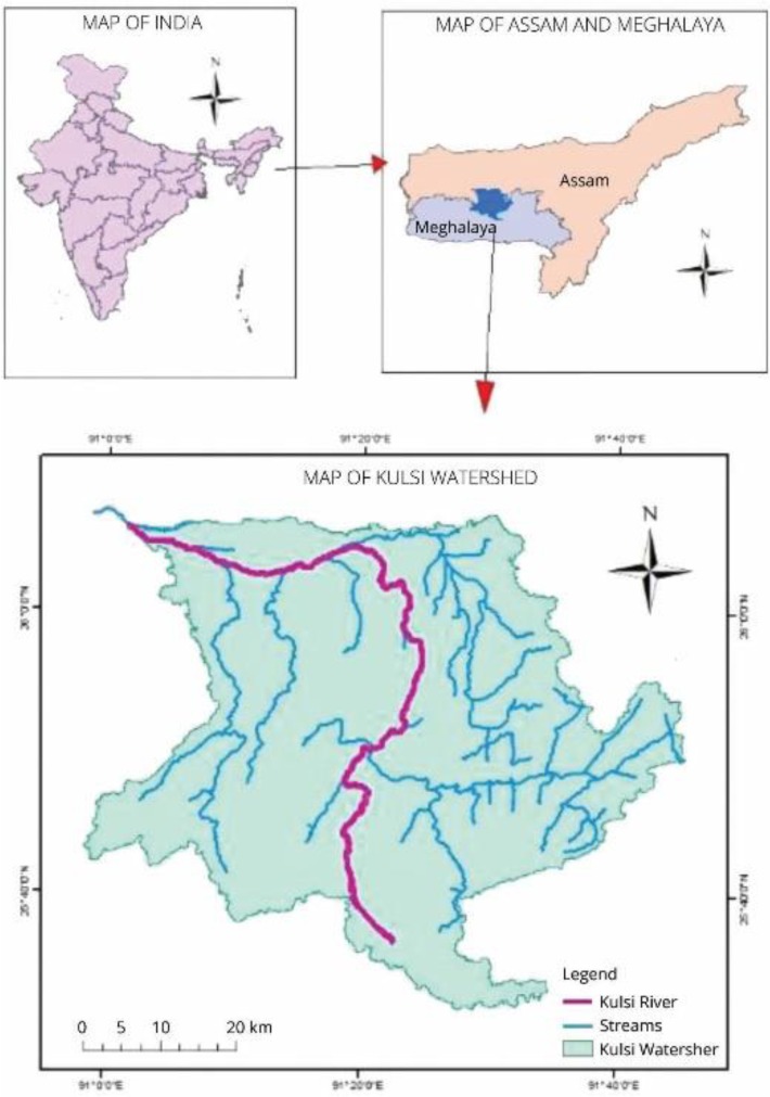
In this study, the Kulsi River Basin, a part of the Brahmaputra sub-basin, was selected and was treated as a hypothetically ungauged basin. A total area of 2822.99 km2 drains through the Kulsi River Basin, covering the Kamrup District of Assam, the Western Khasi Hills, and the Ri Bhoi district of Meghalaya in northeast India. Because of its strategic location (encompassing two states in northeast India) and the fact that the region experiences large floods, the basin is an ideal target for flood routing. The study area is situated on the south bank of the mighty Brahmaputra River. It is located at latitudes 25°30'N to 26°10'N and longitudes 89°50'E to 91°50'E (Fig. 1).
2.2. Data
Daily rainfall data for 2010 were collected from the Indian Metrological Department (IMD), Guwahati. Daily discharge data for 2010 at the basin outlet were collected from the National Institute of Hydrology, Guwahati. Digital elevation models (DEM) are being widely used for watershed delineation, extraction of stream networks, and characterization of watershed topography (elevation map, slope map, and aspect map) by using a watershed delineation tool in ArcGIS software. The DEM used in this project was collected from CartoSat 1_V3_R1. CartoDEM version_3R1 is a national DEM developed by the Indian Space Research Organization (ISRO) with the accuracy of 3.6-4 m (RMSE). CartoDEM version_3R1 has resolution of 30.87 m × 30.87 m (or 1 arc sec). For the delineation of the Kulsi River Watershed, the GeotiffCartoDEMs are ng46g, ng46h, ng46m, and ng46n. In this study, soil data were obtained from the Harmonized World Soil Database v 1.2 of the Food and Agriculture Organization (FAO) soil portal. The Kulsi River Watershed soil texture consists of clay loam, loam, and sandy loam. The study area's soils are categorized into four hydrological classifications (A, B, C, and D) depending on the infiltration rate and other traits. The important soil features affecting the hydrological classification of soils are effective depth of soil, average clay content, infiltration rate, and the soil's absorbing capacity. Group A is low runoff potential, Group B is moderately low runoff potential, Group C is moderately high runoff potential, and Group D is high runoff potential.
2.3. Land Use and Land Cover (LULC)
The LULC for the Kulsi River Watershed was developed by Maximum Likelihood Supervised Image Classification as per the required class sample using ArcGIS 10.1 software. A Linear Imaging Self Scanning Sensor (LISS)-III Satellite image is used in this project to perform supervised image classification. The LISS-III image operates in three spectral bands in Visible and Near Infrared (VNIR) and one band in Short Wave Infrared (SWIR) with 23.5 m spatial resolution and a swath of 141 km. The LISS-III image was downloaded from Bhuvan.
2.4. Sub-Basins of Kulsi River Basin
Eight lateral inflows have been identified as contributing to the mainstem Kulsi River. Sub-basins for lateral inflows are delineated using ArcGIS 10.1, and the details of each sub-basin are presented in Table 1.
Table 1.
Details of the sub-basins of the study area.
2.5. Rainfall data distribution
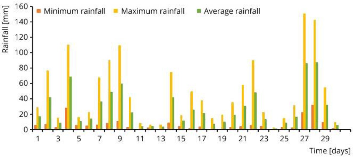
Rainfall distribution over the study area was estimated by the interpolation method using ArcGIS software. Inverse Distance Weighted (IDW), Kriging, and Spline are the three general methods available in Arc GIS 10.1 for interpolation. In this study, the IDW method was used for rainfall interpolation as IDW is the best for the point data format.
The field rainfall data is collected from seven numbered rain gauge stations around the Kulsi Watershed. In 2010, the month of June experienced a maximum amount of rainfall. For this study, daily rainfall for the month of June 2010 is distributed over the study area using IDW using ArcGIS 10.1. The minimum and maximum daily rainfall data for the month of June are presented in Figure 2.
3. Methodology
3.1. SCS-CN method
In this study, SCS-CN is used as a rainfall-runoff model to obtain an inflow hydrograph upstream of the ungauged basin. This method is a simple, predictable, and stable conceptual technique for estimating direct runoff depth based on storm precipitation depth. It relies on only one parameter, the Curve Number (CN). Currently, it is a well-established method, having been widely accepted for use in India and many other countries.
The SCS-CN method is based on the water balance equation and two fundamental hypotheses. The first hypothesis is that the ratio of the amount of direct surface runoff Q to the total precipitation P (or maximum potential surface runoff) is equal to the ratio of the amount of infiltration Fc to the amount of the maximum potential retention S. The second hypothesis is that the initial abstraction Ia is some fraction of the maximum potential retention ‘S’ (Subramanya 2008).
Water balance equation:
Proportional equality hypothesis:
Ia is some fraction of the potential maximum retention (S):
where: P is the total precipitation; Ia the initial abstraction; Fc the cumulative infiltration excluding Ia; Q the direct surface runoff; S the potential maximum retention or infiltration, and λ the regional parameter dependent on geological and climatic factors (0.1 < λ < 0.3).
Solving Equation (2):
By analyzing the rainfall and runoff data from small experimental watersheds, the relationship between Ia and S was established and expressed as Ia = 0.2S. Combining the water balance equation and proportional equality hypothesis; the SCS-CN method is represented as:
A Curve Number (CN), which is a function of land use, land treatments, soil type, and antecedent moisture condition of the watershed, is correlated with the potential maximum retention storage S of the watershed. The Curve Number is dimensionless and ranges from 0 to 100 in magnitude. Using equation (7), the S-value can be obtained from CN in mm.
3.1.1. Curve Number (CN)
The hydrological classification is adopted in the determination of CN. Based on the infiltration and other characteristics, soils are classified into classes A, B, C, and D in order of increasing runoff potential. Effective soil depth, average clay content, infiltration characteristics, and permeability are the important soil characteristics which influence the hydrological classification of soils. In this study, the variation of curve number for various land conditions and for different hydrological classification is obtained from Chow et al. (1988).
3.2. Modified Cunge-Muskingum method
Cunge (1969) proposed the Cunge-Muskingum method based on the Muskingum method, a method traditionally applied to linear hydrologic storage routing. Referring to the time-space computational grid shown in Figure 3, the Muskingum routing equation is modified and written as equation (8), for the discharge at x = (i + 1)Δx and t = (j + 1)Δt:
Where C0, C1, and C2 are the routing coefficients.
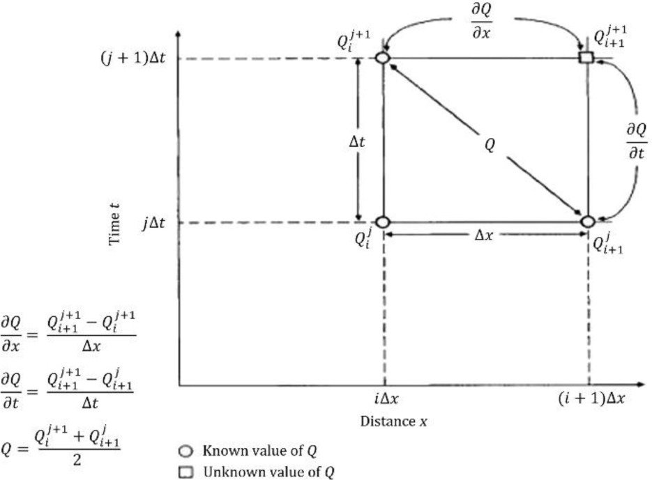
In equation (9) through (11), K is a storage constant having dimensions of time and X is a factor expressing the relative influence of inflow on storage levels. Equation 8 gives an approximate solution of a modified diffusion equation:
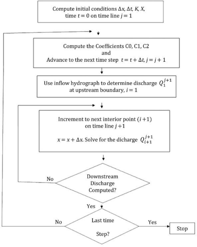
Where ck is the celerity of wave corresponding to Q and B, and B is the top width of the surface water. Cunge (1969) showed that for numerical stability, it is required that 0 ≤ X ≤ 1/2. Figure 4 shows the procedure for the modified Cunge-Muskingum method adopted in the present study.
4. Results and discussion
4.1. SCS-CN Rainfall-Runoff Model in the Kulsi River Basin
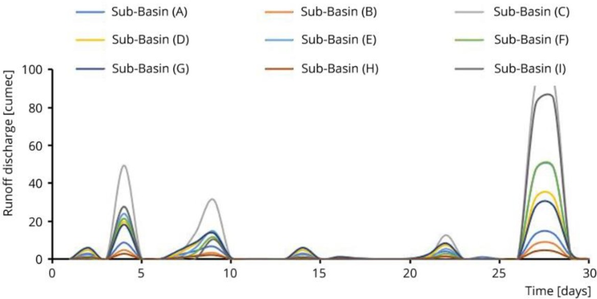
Flood routing is a process to determine the outflow hydrograph at a point on a watercourse from the known inflow hydrograph at the upstream gauged station. The flood routing process is difficult in ungauged basins due to a lack of data. In this study, the SCS-CN model is used to obtain the inflow hydrograph at the upstream section (Ukiam Dam Site). Similarly, the lateral inflows of the eight sub-basins contributing to the Kulsi River are also obtained by SCS-CN. The runoff discharge hydrograph for each sub-basin is presented in Figure 5. The figure shows that the peak runoff discharge for each sub-basin occurred on 28 June, 2010. Sub-basin C shows a maximum peak discharge of 95.35 m3/s, whereas sub-basin H shows a minimum peak discharge of 4.31 m3/s. It is also observed that all the lateral inflow hydrographs follow the same trend.
4.2. Criteria for evaluation of model performance
The following criteria were used to evaluate the performance of the model:
1). In order to compare the proposed model output to the data observed, the criteria for making such a comparison must first be identified (Green, Stephenson 1985). In the present study, the difference between the observed and the computed hydrograph was analyzed by root-mean-square error (RMSE). The RMSE evaluates the magnitude of the error in the computed hydrographs (O'Donnell 1985; Schulze et al. 1995) and is given by:
In this equation, Qcomp represents the computed outflow, and Qobs represents the observed outflow.
2). The criterion for the difference between computed and observed peak discharge (Epeak) (Green, Stephenson 1985) is given by:
The above equation shows the percentage of error in the peak discharge. In the present study, the peak flood discharge at the outlet of the basin obtained from the computed flood hydrograph was compared with the observed flood hydrograph. In equation 16, Qp,comp is the computed peak flows in m3/s, and Qp,obs is the observed peak flows in m3/s.
3). The criterion for the difference between computed and observed peak discharge time (Etime) is given by:
The above equation shows the percentage of error in peak discharge time. In the present study, the peak flow time for the computed and observed flood hydrograph was compared. In the above-mentioned equation, tp,comp is the time taken by the computed hydrograph to reach the peak flow in hours, and Qp,obs is the time taken by the observed hydrograph to reach the peak flow in hours.
4). The criterion for the difference between the computed and observed total volume (Evolume) is given by:
The above equation shows the percentage of error in the total volume of the computed hydrograph. In the present study, the total volume was compared for computed and observed flood hydrographs. In the above-mentioned equation, Vcomp is the total volume of the computed hydrograph in m3 and Vobs is the total volume of the observed hydrograph in m3.
5). Relative error (RE) is given by:
The above equation shows the relative error in percentage. In the above-mentioned equation, Qo is the observed data at the time t and Qp is the predicted value at the time t. The relative error is used to determine the percentage of samples belonging to one of the three groups (Corzo, Solomatine 2007):
− RE ≤ 15% low relative error
− 15% < RE ≤35% medium error
− RE > 35% high error
6). Mean absolute error (MAE) (Cheng et al. 2017) is given by:
In the above-mentioned equation n is the number of samples, Qo is the observed data at the time t, and Qp is the predicted value at the time t.
7). Correlation coefficient (r) is given by:
In the above-mentioned equation n is the number of samples, Qo is the observed discharge at the time t, Qp is the predicted discharge at the time t, Qmp is the mean of predicted discharge, and Qm is the mean of observed discharge.
8). Coefficient of efficiency (CE) (Nash, Sutcliffe 1970) is given by:
In the above-mentioned equation n is the number of samples, Qo is the observed data at the time t and Qp is the predicted value at the time t, and Qm is the mean of observed discharge. Moriasi et al. (2007) recommended the following model performance ratings:
− CE ≤ 0.50 unsatisfactory
− 0.50 < CE ≤ 0.65 satisfactory
− 0.65< CE ≤ 0.75 good
− 0.75 < CE ≤ 1 very good
9). Kling-Gupta efficiency (KGE ).
Gupta et al. (2009) developed this goodness-of-fit measure to provide a diagnostically interesting decomposition of the efficiency of Nash-Sutcliffe efficiency, which facilitates the analysis of the relative importance of its various components. In the context of the hydrological modelling Kling et al. (2012), proposed a revised version of this index to ensure that the bias and variability ratios are not cross-correlated.
where: CC is the Pearson correlation coefficient; rm is the average of observed values; cm is the average of predicted values; rd is the standard deviation of observation values; and cd is the standard deviation of predicted values. Rogelis et al. (2016) consider model performance to be ‘poor’ for 0.5 > KGE > 0. Schönfelder et al. (2017) consider negative KGE values as 'not satisfactory.'
4.3. Application of the Modified Cunge-Muskingum method in the Kulsi River Basin
The method was coded in MATLAB software and the Cunge-Muskingum parameters K and X were determined. The computed outflow hydrograph using the proposed model and the observed data (hydrograph) collected from the National Institute of Hydrology (NIH), Guwahati, are presented in Figure 6. From the figure, it can be seen that the shape of the computed outflow hydrograph is very much similar to that of the observed data at the outlet of the Kulsi River Basin.
Fig. 6.
Comparison graph of the observed outflow and the calculated outflow at the Kulsi River outlet for the Cunge-Muskingum method.
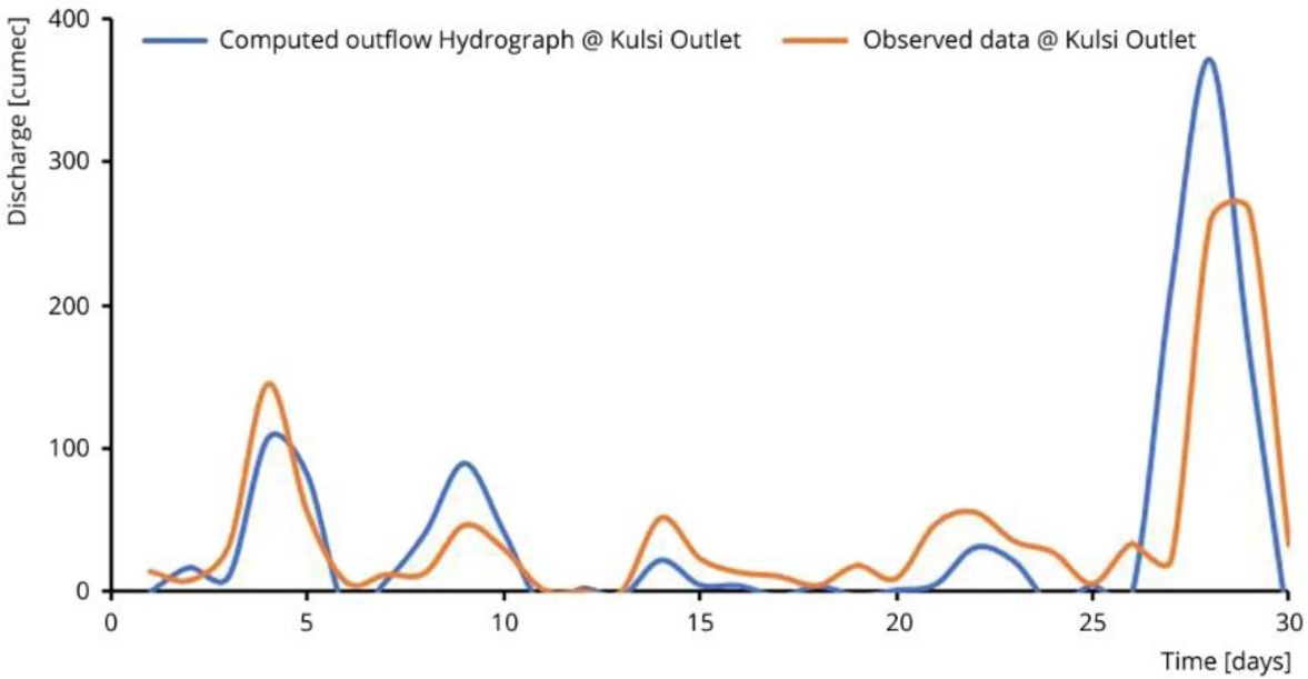
The quantitative comparison of the proposed model with the observed data is presented in Table 2. From the table, the computed peak outflow was on the 28th day, 24 hr prior to the observed peak outflow. The computed peak outflow discharge was greater than the observed outflow discharge. The computed peak discharge was 370.53 m3/s, whereas the observed peak discharge was 265.17 m3/s. The performance of the model is evaluated by nine different criteria, with results presented in Table 2.
Table 2.
Comparison of the performance of the proposed model with the observed data at the outlet of the Kulsi River Basin.
4.4. Sensitivity analyses
The significance of sensitivity studies in modelling is generally acknowledged. Sensitivity analyses allow for the evaluation of the consequences of input errors, and the sensitivity of model parameters relative to other parameters allows for an understanding of the significance of the corresponding inputs (Akbari, Barati 2012).
The Kulsi River Basin was selected to test the sensitivity of the input variables on the output of the proposed model. For this purpose, the upstream hydrograph must be developed for the upstream boundary condition. Figure 7 shows the upstream hydrograph generated in this study using SCS-CN. The sensitivity of the proposed model was determined by varying individual input parameters such as river length, roughness coefficient, bed slope, inflow peak discharge, channel width, and then evaluating the effects on outflow peak discharge, time to peak, velocity, depth corresponding to peak discharge, and volume of the hydrograph.
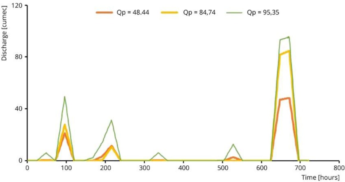
Sensitivity analysis requires basic values for the parameters, which are then adjusted within a given range; the model variance is evaluated for each set of parameter values. Table 3 shows the range of parameter variations based on the features of the Kulsi River and the uncertainty of the model's input parameters. The Sensitivity Index SI (percent) is used for a comprehensive analysis of the impact of changing input parameters on output outcomes in an ungauged basin.
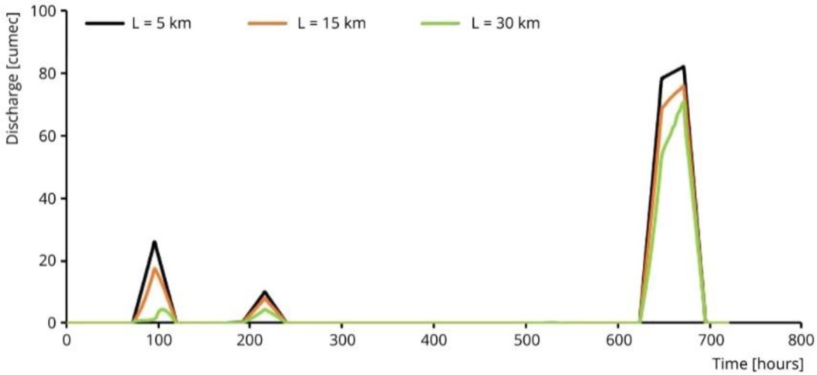
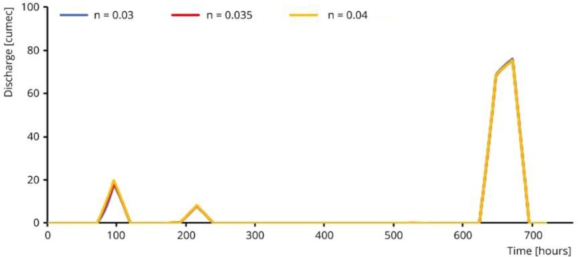
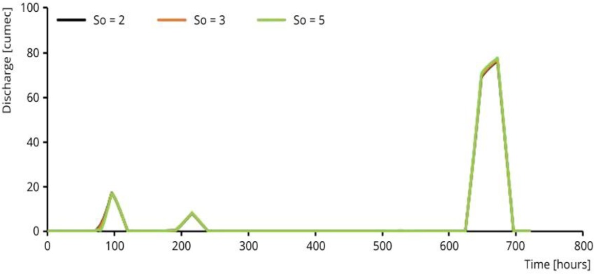
Where I1 and I2 are the smallest and largest values of input parameters, and O1 and O2 are output values corresponding to I1 and I2, respectively. SI is used to compare parameter sensitivities. A negative SI indicates an inverse relationship between input and output parameters (i.e., the output value of the model decreases as the input value increases) (Akbari, Barati 2012). The results of the performance of varied input parameters are presented in Table 4. The SI values for the proposed model were evaluated based on changing one input parameter and evaluating the effect on the selected output result (Table 5). The effects of variations in river length L, roughness n, and bed slope S0 on the output hydrographs are illustrated in Figures 8 to 10, respectively. The figures indicate that river length is the most influential parameter with regard to the shape of the output hydrograph.
Table 3.
Values of parameters for sensitivity analysis of the Modified Cunge-Muskingum method.
| Parameters | Peak flow [m3/s] | Length [km] | Roughness [S/m.^(1/3)] | Bed Slope [m/km] |
|---|---|---|---|---|
| Lower bound | 48.44 | 5 | 0.03 | 2 |
| Base Value | 84.74 | 15 | 0.035 | 3 |
| Upper bound | 95.35 | 30 | 0.04 | 5 |
Table 4.
Performance of the different input parameters.
Table 5.
Values of sensitivity index [%].
| Peak Inflow | Roughness Coefficient | Bed Slope | River Length | |
|---|---|---|---|---|
| Peak outflow | 108.18 | –3.94 | 1.78 | –7.94 |
| Time of Peak | 0.00 | 0.00 | –0.17 | 0.21 |
| Volume | 149.35 | –32.56 | 0.90 | –0.40 |
| Depth | 39.54 | 68.70 | –20.77 | –1.34 |
| Velocity | 71.76 | –73.36 | 22.56 | –1.86 |
4.4.1. Discussion of results
Sensitivity index
Based on the Modified Cunge-Muskingum method sensitivity assessments, this section highlights the relevant input parameters for each of the output outcomes. Table 6 shows the result of the parameter importance rankings.
Table 6.
Sensitivity rankings of the inputs to the MDWMP: P, peak inflow; n, roughness coefficient; L, river length; S, bed slope.
| Order of importance | Peak outflow | Time to peak | Volume | Depth | Velocity | All parameters |
|---|---|---|---|---|---|---|
| 1 | P | L | P | n | n | P |
| 2 | L | n | n | P | P | n |
| 3 | n | -- | S | S | S | S |
| 4 | S | -- | L | L | L | L |
According to the SI findings for peak outflow, the following parameters are ranked in order of importance: peak inflow, river length, roughness coefficient, and bed slope. Although the SI of the peak outflow is modest for bed slope, it is substantial for the other parameters. According to the sensitivity index, the peak discharge has an inverse connection with the roughness coefficient and river length.
The SI results for the period of peak show that river length and bed slope are the most important parameters. For peak inflow and roughness coefficient, however, the SI of the peak time is insignificant. In contrast to the bed slope, the river length has a direct relationship with the time of the peak. The SI results show that peak input, roughness coefficient, bed slope, and river length are the most important parameters for flood volume. In contrast to the roughness coefficient and river length, the peak inflow and bed slope have a direct connection with volume. The SI results show that the roughness coefficient, peak inflow, bed slope, and river length are the most important parameters for the depth corresponding to the peak discharge. The peak inflow and roughness coefficient, unlike the other parameters, have a direct connection with depth. The SI findings for the velocity corresponding to the peak discharge show that the following parameters are ranked in order of importance: roughness coefficient, peak inflow, bed slope, and river length. Peak inflow and bed slope were shown to have a direct connection with velocity, but roughness coefficient and river length had an inverse association with velocity.
If all output parameters are considered at the same time, the rankings of parameters important for the absolute SI mean are peak inflow (73.76%), roughness coefficient (35.71%), bed slope (9.24%), and river length (2.34%). The strongest effects of the input parameter related to flood characteristics (i.e., peak inflow) are on the volume of the floods and peak outflow, and the strongest effects of the input parameter related to bed surface (i.e., bed slope) are on the velocity and depth, according to the analysis of the SI values. The peak outflow, velocity, and depth are the most affected by the input parameters relating to river geometry (i.e. river length).
Effect of grid size
Numerical tests are used to examine the impacts of grid size (i.e., space and time steps) on the output results in terms of the dimensionless peak discharge. The impacts of changing time and spatial steps on the proposed model's performance were explored in these experiments. This method was carried out using the inflow hydrograph at the Kulsi River's entrance. Figures 11 and 12 show variations in the peak of the outflow hydrograph ordinate Qpo, which was dimensionless, and the peak of the inflow hydrograph ordinate Qpi with variations in space and time steps.
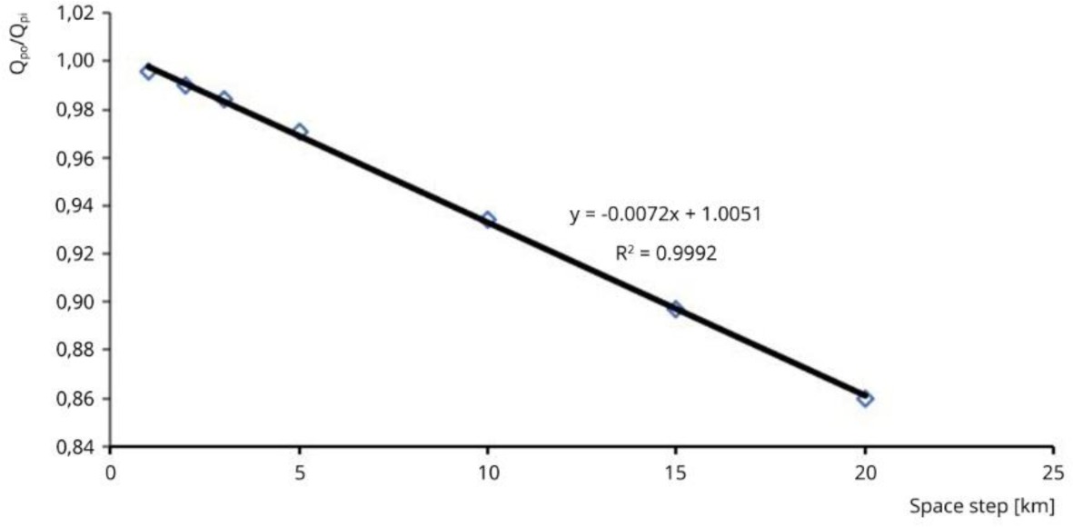
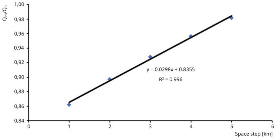
Both the space step and the time step with the peak discharge were found to have a linear connection with a high correlation coefficient. Based on the numerical data, it can be said that differences in time step have only a little influence on peak discharge and have no effect on time to peak. The effects of changes in the space step on the peak discharge are more substantial than the impacts of variations in the time step.
5. Conclusion
In the present study, the inflow hydrograph and lateral inflow hydrographs of the Kulsi River Basin are obtained using the SCS-CN rainfall-runoff model. The modified Cunge-Muskingum model is employed to anticipate the outflow hydrograph at the outlet of the Kulsi River Basin. One of the advantages of the proposed approach is that the outflow hydrograph is obtained through a linear algebraic equation instead of a finite difference scheme or characteristic approximation. This allows the entire hydrograph to be obtained at the required cross-section, whereas in the other models, requiring a solution over the entire length of the channel for each time step. The modified Cunge-Muskingum method allows more flexibility to choose time and space increments for the computations. The results obtained by using the proposed model shows good agreement between the computed and observed outflow hydrograph at the outlet of the Kulsi River Basin. The performance of the model is also assessed considering nine statistical parameters namely RMSE (50.34 m3/s), peak flow error (39.73%), peak flow time error (–3.44%), total volume error (7.36%), relative error (7.36%), mean absolute error (33.5%), correlation coefficient (0.785), Coefficient of efficiency (0.59) and Kling-Gupta efficiency (0.66). Based on the performance of the proposed model, it is concluded that the model can be efficiently used to predict the outflow hydrograph in an ungauged basin. A sensitivity analysis of the proposed model was performed to understand the reliability of the computed outputs in order to make effective decisions when developing a model to simulate the natural process. This study demonstrated that in the selection of input parameters, parameters with a high sensitivity index (SI) must be identified. The impact of grid size on output outcomes has also been studied. The results demonstrate that differences in space step have a greater influence on peak discharge than variations in time step. Some of the improvements which can be incorporated in the proposed model are summarized below.
1). In the present study an established mathematical equation is used for estimating the Muskingum Coefficient. Linear programming, genetic algorithms, fuzzy inference system, radial basis function, and other advanced neurocomputing techniques can be explored to improve the performance of the proposed model.
2). The present study employed rainfall of June 2010. More rainfall events may be analyzed as and when sufficient data become available to make the forecasting more robust and reliable.
3). The proposed model can be improved by using the modified SCS-CN method as a rainfall-runoff model.