1. Introduction
Monitoring surface water quality provides important information that can be used for actions to sustain ecological systems, as well as to protect human health and livelihoods. Assessing temporal and spatial changes in water quality is fundamental for controlling and preventing water pollution. Several approaches have been investigated over the years to analyze such changes. Traditional methods based on statistical and numerical models are structurally complex, costly, time consuming, and require substantial data and detailed information (Jadhav et al. 2015). In addition, traditional models are not capable of reflecting the sophisticated interaction between chemical, physical, and biological properties of water quality (Chen et al. 2018). Furthermore, traditional models often require data pre-processing and assumptions regarding statistical distribution of data, which is usually unknown (Najah et al. 2019).
Recent developments in computer science, especially in Artificial Intelligence (AI), overcome most limitations of traditional modeling and has shown potential for handling water quality data (Tiyasha, Yaseen 2020). Machine learning (ML) is a branch of AI that enables computers to learn without explicit programming (Mitchell 2013). ML has been widely used in many fields, including medicine (Long et al. 1993), engineering (Hulten 2018), finance (Mezrich 1994), ecology (Kijewski et al. 2019), as well as environmental and water resources engineering (Chen et al. 2018; Norouzi, Moghaddam 2020). One of the powerful features of ML is its capability to identify non-linear and complex relationships between input and output data (Najah et al. 2019). Several ML models have been applied to water quality studies over the past two decades, including neural networks (Yu et al. 2020), artificial neural networks (Jeong et al. 2001; Amiri, Nakane 2009; Imani et al. 2021), adaptive neuro-fuzzy inference systems (Najah et al. 2019), support vector regression models (Wang et al. 2017), and rough set theory (Zavareh, Maggioni 2018). Some ML algorithms, including factor analysis (Akoto, Abankwa 2014), principal component analysis (PCA) and granger causality (Zavareh et al. 2021), have also been explored for data dimension reduction and to identify causal relationships. However, none of these techniques is perfect. For example, artificial neural networks require large amounts of data for training and often overfit data (Tiyasha, Yaseen 2020). On the other hand, approaches like rough set and fuzzy set theories cannot handle and/or process quantitative data (Dubois, Prade 1992). Data dimension reduction techniques, like PCA, can make it difficult to interpret principal components (Karamizadeh et al. 2013).
Within ML forecasting models, RF is appealing because (Díaz-Uriarte, Alvarez de Andrés 2006; Boulesteix et al. 2012): (a) RF handles quantitative as well as qualitative data; (b) it does not overfit data; (c) its predictive performance is high compared to other modeling approaches; (d) it can directly process high dimensional data without dimensional reduction; (e) it does not need pre-processing; and (f) it can capture non-linear dependencies between predictor and predicted variables.
RF has been employed in water resources science and engineering in recent years (Parkhurst et al. 2005; Chen et al. 2017; Tyralis et al. 2019; Li et al. 2020). For instance, RF models have proven successful in generating groundwater potential maps (Golkarian et al. 2018; Sameen et al. 2019), stream flow forecasting (Papacharalampous, Tyralis 2018), predicting groundwater level (Wang et al. 2018), analyzing effects of urbanization on hydrological variables (Saadi et al. 2019), urban water consumption forecasting (Chen et al. 2017), as well as for predicting water inrush rate in coal mines (Zhao et al. 2018) and soil infiltration rate (Singh et al. 2017). RF is particularly suitable when non-linear relationships exist, which is the case for the majority of processes in water science (Kijewski et al. 2019; Tyralis et al. 2019).
RF has also become popular for predicting water quality indicators (Papacharalampous, Tyralis 2018). For instance, Devi (2019) investigated the application of an RF classification model to water quality prediction in Kadapa district, India. The study examined water quality indicators, including pH, total dissolved solids, electrical conductivity, and chloride concentration to build a Water Quality Index (WQI) for drinking water assessment, revealing that total dissolved solids was the most important variable affecting WQI, whereas pH was least important. The model classified drinking water in the region with 94% accuracy and a 6.3% error rate. Another study investigated the application of an RF classification model on water quality (Tesoriero et al. 2017) to predict redox-sensitive contaminant concentration (nitrate, iron, and arsenic) in groundwater in northeastern Wisconsin. Their RF classification showed a high potential for assessing aquifer and stream vulnerability at regional and national scales. Furthermore, Wang et al. (2021) developed an RF regression model to predict water quality distribution in China’s Taihu Lake basin. Their model used watershed features and climate variables as predictor variables of three water quality parameters, permanganate index (CODMn), total phosphorus (TP), and total nitrogen (TN). The RF models showed that TN concentration was affected by agricultural non-point sources, while the CODMn and TP were impacted by agricultural and domestic sources.
The present work builds upon these past studies and develops an RF regression model to assess water quality indicators in selected watersheds within Chesapeake Bay basin in the Eastern United States. Different scenarios are proposed to evaluate the effect of different groups of predictors on model performance and to rank their importance in estimating several major water quality indicators: dissolved oxygen concentration, specific conductivity, and turbidity. Finally, an independent watershed is used to assess the transferability of the proposed RF model to other watersheds having similar climate, size, and topography.
2. Study area and dataset
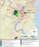
Eleven watersheds across the District of Columbia, Maryland, and Virginia (known as the DMV region) were selected for this study. The DMV region is particularly vulnerable to hydro-meteorological hazards, which are exacerbated by sea level rise because of its vicinity to the coast (Solakian et al. 2020). In addition, excessive algal growth, poor water clarity, and low dissolved oxygen related to eutrophication have been issues in the Chesapeake Bay area for the past few years (Zhang et al. 2018). Thus, researchers, local organizations, and governmental agencies have increased their efforts to collect and interpret water quality data to promote the health of the DMV watersheds that feed into the bay (Zhang et al. 2018).
Data for this work are extracted from 11 United States Geological Survey (USGS) stations located at the outlet of each watershed, as shown in Figure 1. These data contain water quality indicators, including dissolved oxygen (DO) in milligram per liter (mg l-1), specific conductivity (K) in microsiemens per centimeter at 25 degrees Celsius (µS cm-1 at 25°C), turbidity (Tu) in Formazin Nephelometric Units (FNU), and water temperature (WT) in degrees Celsius (°C). Additional information is also considered here, including precipitation, discharge, air temperature, watershed size, and length of rivers running across watersheds, along with watershed land cover, soil type, and livestock count. These data are mainly extracted from USGS, National Aeronautics and Space Administration (NASA), North America Land Data Assimilation System (NLDAS), and National Land Cover Database (NLCD). For more information regarding the data and the watersheds, we refer the reader to Zavareh et al. (2021).
Table 1 displays watershed characteristics, including watershed physiology (size of watershed and total length of rivers in a watershed), land cover, soil type, and livestock head count for all watersheds in this study. Water-sheds 1-10 are used for developing the RF model, whereas Scotts Level Branch (watershed 11) is used as an independent watershed for assessing model performance in the validation phase of this study.
Table 1.
Characteristics of watersheds in this study. Watershed area and total length of rivers are in km and km2, respectively, whereas land use and soil type are in percent.
Watershed size varies between 7 and 169 km2, while the total length of rivers ranges between 5 and 132 km. Land cover is summarized into five main groups, including wetland, developed, barren, forest, shrubland, and reported as percentages. Most watersheds are highly urbanized, with more than 50% of the total area being developed, except for watersheds 4 and 10. Watershed 4 is least developed, with only 8% of its total area classified as developed; watershed 6 is the most developed, with 87% of the total area classified as developed. Four watersheds (1, 4, 5, and 6) are mainly characterized by soil type B with moderate infiltration, whereas there is a prevalence of soil type C with slow infiltration in all other watersheds. Soil type is A least common in all watersheds. Land use and soil type affect infiltration rates, stream flow, and stormwater runoff (carrying contaminants), and can be particularly useful for interpreting relationships among water quality indicators and environmental characteristics (Zavareh et al. 2021).
The minimum and maximum livestock head counts were 2 and 885, respectively. As shown in Table 1, even highly urbanized watersheds contain livestock (e.g., watershed 6 is the most urbanized watershed and has a headcount of 89 livestock). The livestock head count is included because the manure and waste from concentrated animal feeding operations have been a long-standing concern in contamination of water runoff as a potential non-point source of water quality degradation (Burkholder et al. 2007; Dufour et al. 2012).
3. Methodology
3.1. The Random Forest Model
RF is an ensemble method, first developed by Breiman (2001), that uses multiple decision tree algorithms to produce repeated predictions of the same phenomenon. The ensemble combines predictions from multiple learning models to obtain better accuracy than the individual models (Rokach 2010). One of the advantages of the RF method is that there is no need to pre-process or normalize data.
RF can be used for classification purposes and as a regression method depending on the nature of the dependent predicted variable (Tyralis et al. 2019). In regression models, the dependent variable is continuous (quantitative), whereas in classification algorithms it is categorical. RF models for regression are formed by growing trees depending on numerical values as opposed to class labels (Breiman 2001). In the present case, since the nature of predicted variables is continuous, we use an RF regression model. In this approach, RF grows a forest from many regression trees. A Regression Tree (RT) is a set of restrictions or conditions which are hierarchically structured, and which are successively applied from a root to a terminal node or leaf of the tree (Breiman et al. 1993; Zabihi et al. 2016).
The first step in developing an RF model is bootstrapping, in which data is randomly sampled from the entire dataset with replacement (i.e., data can be picked more than once). Each RT is grown in a bootstrapped sub-sample of a training dataset, which is known as bagging (Lagomarsino et al. 2017). The remaining data are called Out Of Bag (OOB), and they are used to estimate the prediction error and the importance of the variables (Han et al. 2016). Predictions based on the OOB set prevent overfitting (Lagomarsino et al. 2017). Over-fitting may also result from extremely large trees, where lower branches introduce modeling noise. To avoid overfitting, the RT needs to be pruned. Pruning trees generates a simpler tree by deleting redundant variables. The second step is feature (variable) selection. In order to determine a split at each node in a decision tree, variables are randomly selected as features (Breiman 2001). Feature selection helps to build uncorrelated trees. Additional, feature selection introduces an extra layer of randomness to the model. The third step is to repeat steps 1 and 2 to build a forest with many trees, with each tree trained with different data. Consequently, two important parameters need to be selected in every RF model: the number of trees and the number of splits at each node.
In this work, the RF model is developed based on data from 10 watersheds across the study area to estimate three water quality indicators: DO, K, and Tu. When one indicator is assigned to be the predicted variable, the other two are used as predictor variables. From the original data, 70% is dedicated to train the model, and the remaining 30% is used for testing (verification). The model is then validated using an independent watershed, i.e., Scotts Level Branch.
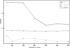
The RF model built based on all information (water quality indicators in addition to information listed in Table 1) is trained with different numbers of trees: 50, 100, 200, 300, 400, 500, and 600 (Fig. 2). The optimal number of trees is chosen based on the value minimizing the relative Root Mean Square Error (rRMSE), which is a measure of the relative misfit between modeled variables (DO, K, and Tu) and the corresponding observed values. This study uses 500 trees, the value at about which rRMSE reaches a plateau. This estimate is consistent with the default values used in prior studies (Boulesteix et al. 2012; Devi 2019; Saadi et al. 2019; Al-Abadi et al. 2021).
Fig. 2.
Values of rRMSE for modeled DO, K, and Tu with respect to their corresponding observed values as a function of the number of trees used in the RF regression model.
Another parameter to calibrate when building an RF model is the number of variables at each split (mtry). For a regression RF model, mtry is suggested to be approximately one third of the number of variables in the dataset (Díaz-Uriarte, Alvarez de Andrés 2006; Boulesteix et al. 2012; Fox et al. 2020). This value was chosen for the present study. Here, mtry values are selected based on the number of variables in each of the six scenarios described in the Section 3.2.
3.2. Model scenarios and performance evaluation
The RF is developed for six scenarios, shown in Table 2. The number of variables increases moving from scenario 1 to scenario 6. The first scenario contains only four water quality indicators, i.e., DO, K, Tu, and WT. In the second scenario, hydrologic characteristics of the watersheds, namely precipitation, discharge, and temperature, are added to the variables considered in scenario 1. In the third scenario, watershed physiology (watershed area and the total length of rivers in each watershed) is included. Land cover information is included in scenario 4, soil type is added to scenario 5, and livestock head count in each watershed is incorporated in scenario 6. As mentioned previously, the number of mtry for each scenario is one third of the number of variables in each scenario: mtry is 2 for scenarios 1 and 2, 3 for scenarios 3, 4 for scenario 4, and 6 for scenarios 5 and 6.
Table 2.
Scenarios and number of predictor variables.
Three statistical metrics are used to analyze model performance of each scenario: correlation coefficient (R) , relative Root Mean Square Error (rRMSE) , and percentage variance explained (%Var).
The correlation coefficient between observed and predicted values is:
where: Vi are the measured values of variables, Pi are the predicted variable values, n is the number of variables in testing data, and
The RMSE indicates the overall misfit between the modeled and observed variables (Yu et al. 2020). This is a common metric to evaluate the performance of prediction results. A perfect prediction model would have zero RMSE. Since the errors are squared before they are averaged, it is very sensitive to large errors in the measured data (Wang et al. 2018). As a result, this study uses rRMSE to assess model misfit. Its calculation formula is:
where: Vi are variables from measured testing data, Pi are predicted values of a variable, n is the number of variables in testing data, and
The %Var is a measure to show how well out-of-bag predictions explain the predicted variance of the training set. The percent variation is the explained variation divided by total variation. In other words:
where: oi is a variable from OOB data, bi is a variable from bootstrap data, and
The importance measure is used to estimate how much the prediction error increases when OOB data for that variable are permuted, while all others are unchanged (Liaw, Wiener 2002). The importance measures are computed to rank all predictors: if the importance measure of a variable is lower relative to others, that variable contributes minimally to the prediction process and can be potentially excluded. The importance measure is computed as the Mean Decrease in Accuracy (MDA) :
where: ntree is the number of trees, EPtj is the OOB error on tree t after permuting the values of Xj, and Etj is the OOB error on the tree t before permuting the value of Xj (Han et al. 2016). Permutation-based importance is crucial since it avoids allocating high importance to features that may not be predictive for unseen data due to overfitting (Pedregosa et al. 2011).
4. Results
4.1. RF Model Evaluation
The three-performance metrics (R, %Var, and rRMSE) are calculated for each scenario when either DO, K, or Tu, is the predicted variable (Fig. 3). The best performance in terms of all three statistics is observed when estimating DO, based on the other water quality indicators. Minimal changes are observed when more predictors are included in the RF model, with slight improvement in %Var and rRMSE when moving from scenario 1 to scenario 2, which added information about watershed hydrology. The effect of urbanization was also significant when DO was granger caused by K and Tu, as shown by Zavareh et al. (2021).
Fig. 3.
Correlation coefficient (top), Explained Variance (middle), and rRMSE (bottom) of DO, K, and Tu with respect to their corresponding observed values for the model scenarios in Table 2.
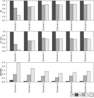
When predicating K and Tu, R values improve when moving to more complex scenarios. This is particularly evident when estimating Tu after hydrological information is added in scenario 2. This can be associated with K and Tu being strongly affected by precipitation and discharge.
In terms of %Var, increases of 20% and 45% are shown for K and Tu, respectively, when information on watershed hydrology is included. In addition, increases of 12% and 10% for K and Tu are detected when water-shed physiology is added to scenario 2. This suggests that hydrological information and watershed physiology highly improve prediction of data variance. However, adding watershed characteristics of land cover or soil type does not improve %Var.
A slight improvement in the rRMSE of DO is observed when hydrologic information is added to the model. When K (Tu) is the predicted variable, rRMSE decreases by more than 50% (140%) when watershed physiology and land cover are added to the model.
Based on these results, the model based on scenario 4, which considers water quality, hydrologic information, watershed size, length of rivers, and land cover, outperforms the other models when considering both the statistical metrics shown in Figure 2 and model efficiency, i.e., the amount of required information. Thus, adding information regarding soil type and livestock count does not improve R, %Var, and/or rRMSE enough to justify the collection of these data, which can be time consuming and expensive in an operational setting. As a result, scenario 4 is selected for further investigation and recommended as the best compromise between performance and efficiency.
4.2. Predictor importance
The importance measures (MDA) for each predicted variable are calculated for every scenario. Higher MDA values indicate when a predictor variable plays a more important role in estimating the predicted variable. In other words, if the accuracy of the RF model decreases due to exclusion of a certain predictor, the predictor is critical in developing the RF model.
Figure 4 shows the MDA values for scenario 4. When predicting DO, WT is the most important variable, followed by discharge and developed area. It is well known that DO and WT are highly correlated (Galloway 2002). A higher volume of water moves faster and increases the flow turbulence, which results in more oxygen dissolving in the water (Kelly 1997). Also, urbanization results in less impervious surfaces, which increase runoff and can elevate the amount of organic matter in water. Consequently, urbanization alters DO concentration due to organic matter decomposition (Smith et al. 1992).
Fig. 4.
Mean decrease in accuracy for predictors of the RF regression model built for Scenario 4 for predicting a) DO, b) K, and c) Tu.
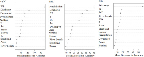
Precipitation is the most important variable for predicting K. This is expected as precipitation increases runoff that can carry saline-polluted water, resulting in higher K. In addition, it is important to note that discharge, WT, and T are also highly predictive of K. This is consistent with findings from Zavareh et al. (2021). The most important watershed characteristic for predicting K is the area of developed land (urbanization). Like precipitation, urbanization contributes to K, as it decreases the possibility of salinity absorption into the soil and increases salinity in surface water.
Discharge is the most important predictor of Tu. Higher water volume increases the speed of its movement, stirring up the water and increasing turbidity (Dalwadi, Padole 2019). The levels of K and WT are the second and third most important variables predicting Tu. This is in line with past studies that have shown strong Granger causality relationships between WT (cause) and Tu (effect) (Zavareh et al. 2021).
In summary, discharge plays a very important role when predicting DO, K, and Tu. Additionally, the volume of discharge is directly affected by land cover. If the land cover of a watershed changes, the overall water yield (runoff) of the watershed changes, which affects water quality (Kumar et al. 2018). This explains why scenario 4 outperforms scenarios 1-3 (which lack information regarding land use, which may have a critical effect on water quality).
4.3. Model validation
In order to assess the applicability of the RF model, we evaluate its performance across an independent water-shed, Scotts Level Branch, for which four months of data are available (January 2020 to April 2020). Information on DO was unavailable for this watershed.
Figure 5 shows time series of predicted and corresponding measured values of K and Tu for Scotts Level Branch. Model estimates are presented for the 6 scenarios as an ensemble envelope bounded by the minimum and maximum values obtained across all 6 models.
Fig. 5.
Time series of modeled and observed K and Tu for Scotts Level Branch. The ensemble of modeled values is shown as a shaded area enveloped between the minimum and maximum values obtained from the models built on the 6 scenarios.
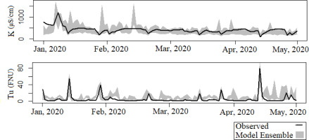
Observed K values fall within the model ensemble bounds, showing that the model encapsulates the actual values of K and well reproduces its variability over time. However, the model identifies a peak in late February that was not captured by in-situ measurements. This can be either due to an overestimation by the model during a specific precipitation event, or it could be an event missed by the observations. Similarly, some peaks in modeled Tu are not present in the observed time series. Nevertheless, Tu variability during the period of interest is well captured within the model envelope.
Table 3 shows the results for the three statistical metrics used in this study to evaluate the RF model performance for K and Tu in the validation watershed for the 6 scenarios. Correlation coefficients more than doubled when adding hydrology information to scenario 1 for both K and Tu. The R value improves when more information is added to the model, and as in the training phase, it increases sharply when hydrology information is included in the model (i.e., moving from scenario 1 to 2). The %Var values for K and Tu more than doubled and tripled when hydrology and watershed physiology information are added (i.e., scenario 1 vs. scenario 3). Conversely, the results of rRMSE do not consistently increase or decrease as more information is added to the model. However, scenario 4 shows relatively low rRMSE compared to other scenarios. In general, when comparing the three statistical metrics, scenario 4 shows the best performance for predicting K and Tu. This is in line with the results for the RF model, as previously discussed.
Table 3.
Correlation coefficient (R) , Explained Variance (%Var), and rRMSE for predicted and observed K and Tu values in the Scotts Level Branch watershed.
| Scenario | K | Tu | ||||
|---|---|---|---|---|---|---|
| R | %Var | rRMSE | R | %Var | rRMSE | |
| 1 | 0.17 | 0.27 | 0.51 | 0.18 | 0.12 | 0.53 |
| 2 | 0.57 | 0.46 | 0.43 | 0.79 | 0.45 | 0.89 |
| 3 | 0.58 | 0.64 | 0.80 | 0.9 | 0.56 | 0.48 |
| 4 | 0.52 | 0.65 | 0.41 | 0.94 | 0.58 | 0.45 |
| 5 | 0.54 | 0.65 | 0.37 | 0.89 | 0.51 | 0.60 |
| 6 | 0.50 | 0.64 | 0.53 | 0.90 | 0.60 | 1.01 |
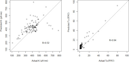
Scatterplots of actual and predicted K and Tu for scenario 4 are presented in Figure 6. Although the dispersion around the 1:1 line is consistent, the modeled K values are overall well aligned to K observed in the watershed during the 4-month validation period, with a correlation coefficient of 0.52. In terms of Tu, the model well reproduces large Tu values (correlation coefficient of 0.94), but overestimates observed values of Tu below 10 FNU. This can be potentially improved by considering a larger sample size and verifying the model for a longer time series and/or in a different watershed.
5. Conclusions
This study investigates the efficiency of RF regression for predicting water quality indicators (DO, K, and Tu) and provides insight into factors affecting stream water quality. The RF models are built based on information from 10 watersheds in the DMV region, with one independent watershed used for assessing model applicability. The RF model performance is analyzed based on three statistical metrics, R, %Var, and rRMSE. In addition, degree of importance is calculated for each scenario to rank relative contribution of predictors in estimating water quality.
The RF models to predict DO show the highest performance (average R = 0.99, average %Var = 0.98, average rRMSE = 0.11) when modeling the 10 watersheds. The RF models predicting K (average R = 0.75, average %Var = 0.57, and average rRMSE = 0.82) slightly outperform the models that predict Tu (average R = 0.69, average %Var = 0.50, and average rRMSE = 1.62). However, when comparing the scenario performances for DO, K, and TU and taking into account the amount of information needed for developing each model, scenario 4 is the most efficient option. This highlights the importance of land cover information in predicting water quality.
The most important measure for predicting DO is WT, which is expected due to their strong correlation (Galloway 2002). The second and third most important measures of DO are discharge and urbanization. In comparison, precipitation and discharge are the most important measures for predicting K. Among all watershed characteristics, urbanization plays the most important role in predicting K, as it results in greater area of impervious land, which increases runoff volume and the concentration of total dissolved solids (Kumar et al. 2018). When predicting Tu, discharge is the most important measure, as more discharge yields more suspended solids, which increases turbidity. The second most important measure is K, as increased dissolved solids concentration contributes to higher Tu.
An independent watershed is used to assess the performance of the developed models and evaluate their applicability to a different region. Model performance is similar to that observed in the training phase, with scenario 4 (which includes water quality data, hydrology information, watershed size, length of rivers in water-sheds, and land cover information) outperforming other scenarios. However, longer time series and different watersheds should be considered to verify these results.
In conclusion, along with watershed physiology and hydrological characteristics, urbanization plays an important role in predicting DO, K, and Tu. In general, land cover highly impacts the production and transportation of sediments and organic matter (Inserillo et al. 2017). This emphasizes the vulnerability of surface water and streams to anthropogenic changes.
It is important to mention that there are limitations in using RF models in water quality data analysis. For instance, extrapolation beyond the training data requires implementing techniques or procedures to mitigate the risks associated with extrapolation, such as using appropriate model validation methods, considering uncertainty estimates, and potentially applying domain knowledge to make informed decision. Additionally, the selection of relevant variables significantly impacts model performance. A comprehensive elucidation of fitting methodologies is imperative to avoid inaccuracy in drawing predictive conclusions.
Future work should extend this study to other regions to verify the effects of climate on the relationships between hydrometeorology and water quality. Additionally, finer temporal resolutions can be considered to investigate rates of hydrological response, especially in watersheds of different sizes. Additional water quality indicators like pH and nitrate concentration would help generalize the results of this work and make the proposed analyses more useful for water quality management. Finally, extreme weather events should be analyzed to understand how they impact model outcomes.

