1. Introduction
Climate change is undeniably confirmed in observational data, regardless of the perspective from which the data is analyzed (FAOSTAT 2022; NOAA 2022). Recognition of the necessity for adaptation and mitigation strategies is evident among governments and societies, a fact substantiated by the initiatives undertaken by the United Nations Framework Convention on Climate Change (UNFCCC). These strategies are rooted in climate data, and their effectiveness hinges on the precision of climate change forecasts. Certain existing climate scenarios fail to depict climate fluctuations for specific regions without accounting for localized conditions.
Precipitation is a meteorological phenomenon characterized by high spatiotemporal variability; unlike temperature or air pressure, this parameter is discontinuous. This makes interpolation or forecasting of precipitation challenging. This work attempts to create a reference field for Poland for the process of adjusting climate scenarios.
Based on The Fifth Assessment Report (IPCC 2014) prepared by the Intergovernmental Panel on Climate Change (IPCC), an international program, the Coordinated Regional Downscaling Experiment (CORDEX) (Giorgi et al. 2009) was established in the frame of the World Climate Research Program (WRCP). The CORDEX aimed to organize and coordinate a framework to produce improved regional climate change projections for 14 regional (CORDEX) domains. Among these 14 domains is EUR-11, which covers Europe. For this region, climate simulations were prepared and developed by the European branch of the international CORDEX initiative (EURO-CORDEX) (Jacob et al. 2014; Benestad et al. 2021). This project offers hindcast simulations, historical simulations, and climate scenarios (Benestad et al. 2017). Hindcast simulations cover 1989-2008, using initial and boundary data from global atmospheric reanalysis produced by the European Centre for Medium-Range Weather Forecasts (ERA-Interim reanalysis) (Dee et al. 2011). They are made for model makers to evaluate the model design and improve it. Historical simulations cover the period of 1951-2005. Regional Climate Models (RCM) use the initial and lateral boundary conditions from Global Climate Models (GCM), and their purpose is to analyze the correctness of the RCM-GCM scheme for a given region. Due to the higher resolution of the RCM model, it is possible to feed the RCM-GCM scheme with a more detailed description of the local environment. For example, height above sea level and terrain type are provided more accurately. As a result, this procedure should make the simulation results closer to real results. Various physical parametrizations and numerical methods are used in RCMs, which means that the quality of past climate reconstructions may change depending on the studied area and model. Comparing historical simulations with the local climate in the studied domain allows for appropriate selection and correction of RCM-GCM schemes. An ensemble of climate scenarios compatible with the domain conditions is necessary to study future climate changes and, in turn, create effective mitigation and adaptation programs.
Reliable and high-quality observational datasets are essential to create good-quality ensembles of climate scenarios. First, the full range of available data, including local observational data, should be used. The resources of many repositories contain gridded datasets, but regional analysis usually does not meet this condition. Within the European Climate Assessment & Dataset project, regular grid data E-OBS (high-resolution gridded mean/max/min temperature, precipitation, and sea level pressure for Europe and Northern Africa) (Cornes et al. 2018) with 0.1- and 0.25-degree spatial resolution and daily temporal resolution are available. The current list of stations from which the observational data are used to create E-OBS sets for rainfall for the territory of Poland includes 1688 items (including 40 synoptic stations provided by the Institute of Meteorology and Water Management – National Research Institute (IMWM-NRI)). However, the period over which individual observation series are available varies significantly. For the analyzed period of 1976-2005, the minimum number of daily records is 89, with a median of 650 (these are significantly lower values than for the data used in this work, for which the minimum is 197 and the median 719). For 1826 days, the number of stations used to create E-OBS reanalysis is less than 197. This corresponds to approximately 17% of the total amount of data in the analyzed period, i.e., approximately five years. The use of more input data can help to describe precipitation more accurately.
Some meteorological services or institutes provide gridded precipitation data, but these have limitations when applied to Poland. The National Oceanic and Atmospheric Administration (NOAA) Physical Sciences Laboratory (PSL) website provides collections with gridded precipitation data ranging from 2.5 to 0.25 degrees. However, the high-resolution collections of gridded precipitation datasets cover only the United States of America (USA) area. The Swiss Federal Institute for Forest, Snow and Landscape Research (WSL) provides free access to high resolution (30 arcsecs, ~1 km) climate data – CHELSA (Climatologies at high resolution for the earth’s land surface areas) (Karger et al. 2017). This website has available data based on a mechanistic statistical downscaling of global reanalysis data or global circulation model output. Unfortunately, the data from the reanalyzes covers the period from 1979, which is already intricate and highly processed.
There are studies where great importance is attached to the maximum use of available observational data, especially when extreme events are important in the analysis, as shown in Sheffield et al. (2006). The study conducted by Belo-Pereira et al. (2011) regarding rainfall data across the Iberian Peninsula demonstrated that accurate descriptions of region-specific meteorological situations require high-resolution datasets derived from a comprehensive measurement network. The global gridded datasets compared in Belo-Pereira et al. (2011) overestimated the number of days with precipitation while underestimating heavy precipitation events.
Two high–resolution daily gridded datasets were created in the climate change impact assessment for selected sectors in Poland (CHASE-PL) project. The work of Berezowski et al. (2016) described the first dataset with a resolution of 5 km covering the period of 1951-2013 for temperature and precipitation in the two largest Polish river basins. The work was carried out by increasing the resolution to 2 km, extending the period from 2013 to 2019, and extending the list of meteorological parameters, including humidity and wind speed (Piniewski et al. 2021). Data from the measurement network of the IMWM-NRI were used, as well as data from all neighboring countries, including the densest data network from Germany. The assessment of the quality of the prepared gridded datasets, included in the works of Berezowski et al. (2016) and Piniewski et al. (2021), also showed that they describe the local meteorological conditions well, but the projected Polish Geographic Coordinate System 1992 (PUWG-92) was used. Many studies (e.g., Herrera et al. 2018; Crespi et al. 2019) on the interpolation of observational data assess the causes of errors, pointing to the role of the density of measuring stations and the properties of interpolation methods. Daly et al. (2017) analyzed the uncertainty in gridded precipitation datasets for densely spaced rain gauge networks in the Appalachian Mountains in western North Carolina, USA. In this study, it was concluded that station density and misallocation are likely sources of errors. The sensitivity assessment of various interpolation methods was included in Crespi et al. (2019), where the 1981-2010 monthly precipitation climatology for Norway at 1 km resolution was presented. In this paper, three interpolation algorithms were considered. The first algorithm, HCLIM+RK (the global historical climate database + Regression Kriging), was a combination of two methods, combining the output from a numerical model with in-situ observations. The second algorithm, MLRK (Multi-Linear Local Regression Kriging), resulted from the Multi-Linear Local Regression Kriging, and the third LWLR (Local Weighted Linear Regression) was the Local Weighted Linear Regression. Among other conclusions from the conducted research, the authors noted that the accuracy of MLRK and LWLR was more sensitive to the spatial variability of station distribution over the domain. Their interpolated fields were more affected by discontinuities and outliers, especially over those areas not covered by the rain-gauge network. A comprehensive analysis of the uncertainty in the gridded data was presented by Herrera et al. (2018). Three factors influencing the quality of the interpolated fields were analyzed: station density, interpolation methodology, and spatial resolution of the fields obtained. In the paper, an experiment was carried out for three interpolation methods and different levels of observational data density. This paper evaluated the experiment’s results with a statistical analysis of variance (von Storch, Zwiers 1999; Deque et al. 2007; 2012). The authors stated that the station’s density explained more than 60% of the variance of the interpolation procedures.
This study aimed to develop reference precipitation gridded datasets covering the territory of Poland. These datasets were planned to evaluate the RCM-GCM ensemble using measures presented in works such as Gleckler et al. (2008) and Konca-Kędzierska (2019), for the last available 30-year period (1976-2005) in the historical simulations on the EUR 0.11° grid.
Several of the works mentioned concerned gridded data for the area of Poland, but they did not correspond to the needs posed in this paper. For example, in Berezowski et al. (2016), Piniewski et al. (2021), and Cornes et al. (2018), a grid other than the EUR 0.11° was considered. In Herrera et al. (2018), the period did not cover the years 1976 and 1977. The undeniable influence of the quantity and quality of observation data on the quality of gridded fields has been confirmed in all these works.
2. Materials and methods
2.1. Data
Given our goal of producing a grid precipitation field for the 1976-2005 period (as part of the EUROCOREX project’s historical scenarios), we opted to rely on the daily precipitation data publicly available from IMWM-NRI1. The IMWM-NRI observation network service department is accountable for ensuring data accuracy, verifying the suitability of station locations, and selecting measurement equipment in compliance with the Technical Regulations of the World Meteorological Organization (WMO). The measurement network includes three types of stations operating in different time regimes: synoptic, climatic, and rainfall. The amount of data for individual days of the period is variable, which affects the interpolated daily fields (Table 1).
Table 1.
The statistics on NDay – the amount of observational data per one day. Min. – minimum of NDay, Mean – average value of NDay, Max. – maximum value of NDay, Q25, Q50, Q75 – 25th, 50th and 75th percentiles of NDay, respectively.
| Stations | Min. | Q25 | Q50 | Mean | Q75 | Max. |
|---|---|---|---|---|---|---|
| Synoptic | 57 | 60 | 60 | 60 | 61 | 63 |
| Climatic | 135 | 142 | 160 | 163 | 174 | 205 |
| Rainfall | 1 | 176 | 505 | 501 | 804 | 1166 |
| All | 197 | 397 | 719 | 717 | 1016 | 1429 |
In the analyzed period, there were 63 days when practically no data from rainfall stations were available, which is less than about 0.6% of the total number of days. In these cases, observations are mainly from synoptic and climatic stations. Although the minimum distance to the neighboring station varies from 3 to 75 km on the day with the lowest number of observations, compared to 0.5 to 33 km on the day with the highest number of observations, the data quality is sufficient, considering data comes from synoptic stations. The number of observations is increased at rainfall stations, densely located in mountainous areas, which undoubtedly significantly increases the quality of reproduction of precipitation by interpolated fields. The density of the observation network, especially in mountainous areas, is crucial for the quality of interpolated fields, e.g., Herrera et al. (2018). As shown in Figure 1, the spatial distribution of the observational data is irregular, which may have uneven effects on the interpolation methods used. The exceptionally high density of the measurement network is characteristic of the mountain and sub–mountain regions, where the spatial variability of precipitation is the highest.
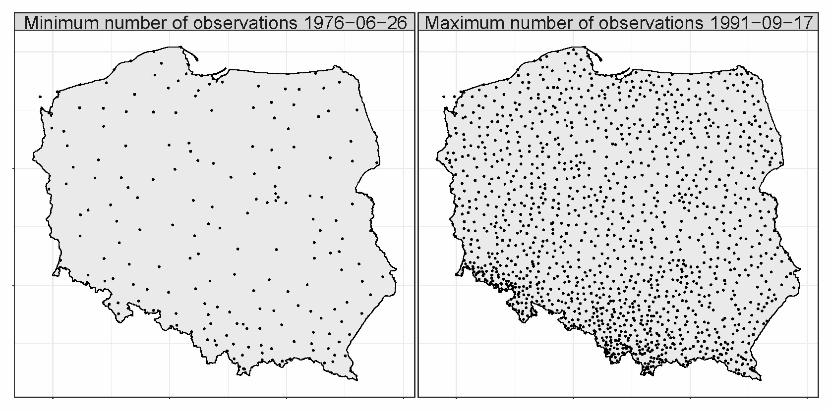
The average annual number of observations per day varied throughout the years, with a median of 719 (ranging from 592 to 821). The variability in the number of observations regarding the type of stations is shown in Figure 2.
Fig. 2.
The average annual amount of data for one day from 1976-2005 for climatic, rainfall, synoptic, and total observations.
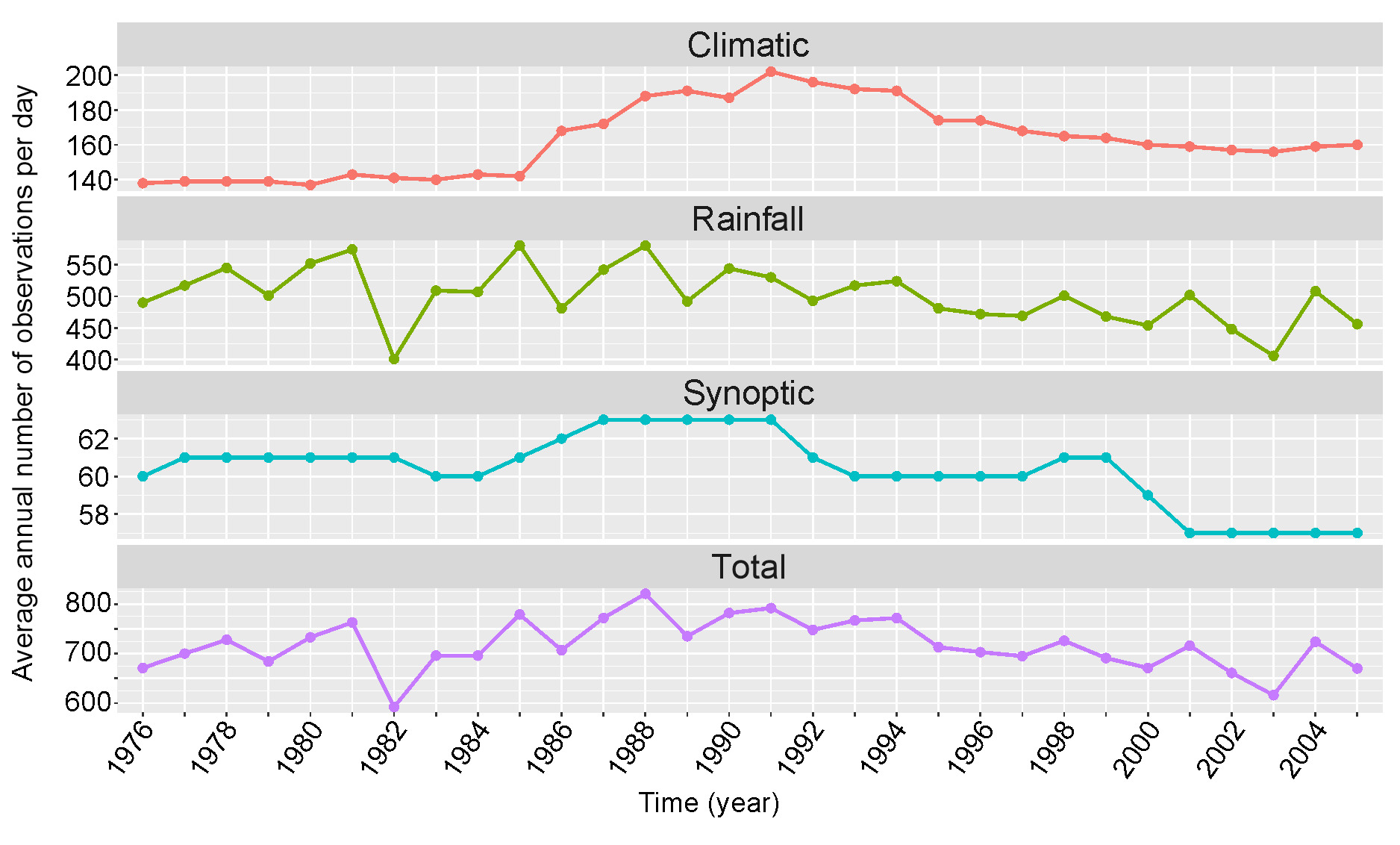
The decrease in the number of synoptic observations was compensated for by the increase in climatic observations, which was related to the change in the type of measurement stations. The number of synoptic stations ranged from 57 to 63; a decrease to 57 occurred in the last years of the period. In the analyzed period, the number of climatic stations increased by approximately 17%, ranging from 137 to 202. Following an increase in the mid-1980s, the number of stations stabilized at 160 by the end of the period. The number of rainfall stations ranged from 401 to 580, and these had the most significant impact on the total number of observations. In this work, we used observation data from IMWM-NRI, which are subject to routine quality control. The local data archive for the analyzed period 1976-2005 was created in November 2019.
2.2. Methods
We utilized the EURO-CORDEX simulation outcomes as-is, thus requiring a reference precipitation dataset that matched the node grid’s shape but was tailored to Poland’s region. Therefore, we selected a domain that is part of the EUR-11 grid. The spatial resolution of the EUR-11 rotated grid is 0.11 degrees, corresponding to a regular grid size of approximately 12.5 km. The analyzed area included only nodes located in Poland, of which there were 2,137. We analyzed the last 30-year period (1976-2005) available in the historical simulations, and will be applied these to correct climate scenarios.
The principle of using all historical data available in the IMWM-NRI database was applied. This caused the number of observations to change significantly on individual days. On the other hand, it is known that interpolation methods are varyingly sensitive to this factor. The combination of both premises suggests that instead of using one sophisticated interpolation method for the entire period, the interpolation method should be selected separately for each day. The allegation of methodological discontinuity can be compensated by obtaining a more realistic and reliable precipitation pattern. The fact that the selected domain is a regular grid with a small step of 0.11 degree influenced the choice of interpolation methods. Deterministic interpolation methods were used, such as bilinear, bicubic, inverse distance weighted, or nearest neighbor. Precipitation observation fields were prepared using the above-mentioned interpolation methods available in the R Project for Statistical Computing (R Core Team 2018) and in the Climate Data Operators tools (CDO) (Schulzweida 2019).
When evaluating interpolation through the leave-p-out cross-validation method (p is the size of the test set), the accuracy of the analysis may be impacted by high variability in the number of observations. Days with a small number of observations (minimum of 197) are assessed less thoroughly than days with many observations (median of 719). The division into training and test sets also introduces randomness into the evaluation process. This could be eliminated by taking as a constant test set the time series for 102 stations for which complete observational data are available. It was decided to abandon the method of dividing the observational data into the training and evaluation part, as it is usually done, for two reasons. Excluding the selected evaluation set from the interpolation process removes the data series most valuable for the interpolation. High variability in the number of observations per day (25% quantile is 397) for 25% of days of the analyzed period would mean resignation from 26% to 52% of the input data for interpolation methods. On the other hand, the leave-one-out computationally expensive method, is a measure of the additional errors incurred during its execution. For each point in the observational data on a given day of the period, interpolation is performed with the value for that point omitted from the input data. Furthermore, the considered point usually does not occur in the target grid, and its value must be somehow calculated (e.g., by choosing the nearest point from the target grid). The cross-validation error is the average of the sum of the additional error in obtaining the interpolated value and the error caused by not considering all points in the input data of the interpolation model. We conducted a comparative analysis of the obtained observation fields for localization, where the complete time series of observations were available during the analyzed period.
The degree of compliance of the obtained fields of observation was assessed based on statistical parameters such as the Pearson correlation coefficient (RO), Root Mean Squared Error (RMSE), and a normalized version of this parameter (NRMSE) as in Belo-Pereira et al. (2011) and Berezowski et al. (2016). In addition, the spatial compliance of the precipitation fields was also examined using the correspondence ratio (CR) (Belo-Pereira et al. 2011). For the obtained reference precipitation fields, the Mean Annual Cycle (MAC), as established in Belo-Pereira et al. (2011), was also compared. The results of the analyses did not allow us to determine the best method among the methods listed in Table 2. Thus, the methods determining the best gridded dataset for particular days based on the correlation coefficient and the correspondence ratio were finally applied and presented in Section 3.10.
Table 2.
Interpolation procedures used.
2.2.1. Interpolation methods
Areas of rainfall are unevenly distributed. The regions with no precipitation can border regions with intense precipitation. This makes precipitation quite a problematic parameter to interpolate. In geostatistics, kriging methods are commonly used, but such an interpolation process sometimes causes problems. In Prasad and Sushma’s (2016) work, the result was satisfactory and encouraging for most of the data. However, where there was a small amount of data, the obtained values exceeded the range of observational data.
We tested several other interpolation methods available in the R environment (R Core Team 2018) and the Climate Data Operators (CDO) (Schulzweida 2019). Table 2 lists the six selected interpolation techniques and the names of the resulting sets with interpolated values.
The interpolation procedures in the Akima package (Akima, Gebhardt 2022) allow for regular and irregular grids for the input data. The method is based on the modified triangulation Akima code. A bilinear interpolation for regular grids was also added for comparison with the bicubic interpolation on regular grids. Calculations are made locally; thus, only neighboring points are considered. In rare cases, the interpolation with a linear function resulted in negative values corrected by the neighboring nodes’ mean value.
The CDO interpolation procedures are based on the Spherical Coordinate Remapping and Interpolation Package (SCRIP) library developed at the Los Alamos National Laboratory (Jones 1998). Both are adapted to interpolate from an irregular grid, such as for measurement grid nodes. By default, the CDO operator ‘remapdis’ uses four values from the nearest neighborhood to interpolate the destination value. The result value is the weighted average of these values, the weights being the reciprocal distance between the points.
Nearest neighbor remapping ‘remapnn’ is the simplest spatial interpolation method. Every predicted point gets the value of the nearest measured point. The fields obtained by this method are not smooth, but they can provide good field interpolation where there is a sufficiently large number of observations.
The ‘gstat’ package is a very rich package for complex geostatic analysis with a scope defined by the title: “Spatial and Spatio-Temporal Geostatistical Modelling, Prediction and Simulation” (Pebesma 2004; Gräler et al. 2016). However, the Inverse Distance Weighted predictions method was selected to prepare the reference field and preserve the similarity of the methods of obtaining the remaining compared fields. The ‘gstat’ package offers implementations of the Inverse Distance Weighted (IDW) method for different values of the power of the distance between nodes. The calculations were performed by utilizing the square of the distance between nodes to determine weights. Introducing this higher power value enhances the influence of values that are near the node. This contrasts with the CDO method known as ‘remapdis’ or ‘Distance–weighted average remapping’, where the distance is not squared.
The last of the selected interpolation methods is the ‘Tps’ procedure from the ‘fields’ package version 11.6 (Nychka et al. 2017). The ‘Tps’ procedure fits a thin plate spline surface to irregularly spaced data, uses a special type of piecewise polynomials, and is expected to give better results. It was applied assuming default parameter values.
2.2.2. Methods of evaluating the obtained reference fields
The obtained reference fields were assessed in three ways: assessment of the general fit based on annual and monthly characteristics; methods of analyzing daily data (in particular, extreme values assessed with number of days in the month when precipitation does not exceed 0.5 mm (LD05) and the 95th percentile (Q95)); and the overall assessment of the fit of fields using illustrative diagrams. Individual parameters were calculated for selected 102 synoptic and climatic stations for which complete data series for the studied period were available.
The first group includes field assessment of the annual sum of precipitation, the annual cycle of the monthly sum of precipitation, and the NRMSE for the monthly sum of precipitation. The overall level of matching reference fields was assessed based on basic statistical characteristics (extreme values, percentiles 1% and 99%, median and Interquartile Range (IQR)) of observational data and reference fields.
The annual cycle of the monthly sum of precipitation was used as described in Belo-Pereira et al. (2011), where the daily gridded precipitation dataset over mainland Portugal was assessed. For stations with complete sequences of monthly rainfall totals, 30–year averages were calculated and compared with the results of corresponding calculations for the reference fields. The percentage difference for the multi-year average of the monthly sum of precipitation allows assessment of the quality of the reconstruction of the annual variability by the reference fields.
To assess the compliance of the precipitation parameters in the interpolated fields, formulas such as the mean absolute error (MAE) were used:
and the mean square error (MSE):
where y is the observation, ŷ is the interpolated value of y, and n is the number of points included in the calculation.
Often, to calculate the error interpolation, the RMSE is used. However, in the case of precipitation, which is a spatially variable parameter, NRMSE may provide a better evaluation measure of interpolation error (Otto 2019).
where σ is the standard deviation of the sample of observations. This allows for assessing the interpolation method, making it independent of local precipitation variability. Using NRMSE, the monthly sum of precipitation, the maximum values, and the quantile of 95% of the daily sum of precipitation in a month were also analyzed. The analysis of cases of absence or very small precipitation was carried out using the number of days per month for which the precipitation was not more than 0.5 mm. The assessment of the spatial fit of reference fields was carried out using the CR, the idea of which was taken from the work Belo-Pereira et al. (2011):
AI is a measure of the intersection of the area where the precipitation in the interpolated field and the field of observation exceeds a given threshold. AU measures the sum of the areas where precipitation in the interpolated field or the field of observation values exceeds a given threshold. The areas for ten thresholds of daily total rainfall from 0.1 mm to 50 mm were analyzed. The number of stations that met this condition over the analyzed period was adopted as a representation of the measure of the investigated areas.
The RO was calculated for the entire period for stations with complete daily sequences of total precipitation. The Pearson correlation coefficient was also calculated for each day in the warm half of the –year (W – months from May to October) and in the cold half of the –year (C – months from November to April).
The mean values of RMSE and MSE for the precipitation statistical parameters listed below were used to construct the ranking of the interpolation methods. For stations with complete daily sequences of total rainfall, the calculated values of MSE and MAE were used for the maximum rainfall in the month (MAX), the monthly sum (MS) of precipitation, the number of days in the month when precipitation does not exceed 0.5 mm (LD05), and the 95th percentile (Q95). The lowest error value gave the highest position in the ranking by summing up the position numbers for individual interpolation methods and all parameters considered (MAX, MS, LD05, Q95). This allowed us to determine which methods provided the best fit using this approach. However, this is too general and a simplified solution, which does not allow for a good interpolation choice in all cases. The interpolation result for individual days depends, to a large extent, on the quantity and quality of available observational data. It is even sensitive to the distribution of data in the domain. The sensitivity of the methods to small amounts of data and not evenly distributed points is very different.
The variance inflation factor (VIF) was analyzed for the 30-year mean of the annual sum of precipitation. This parameter was analyzed in two cases: for interpolation methods (in 3.1 Average annual total of precipitation) and in the case of comparing the result fields of this work with fields from the CHASE projects (in 4. Discussion). For these purposes, a group of 96 stations was selected for which there was no missing data in the years 1976-2005. In addition, stations for which data from the CHASE project could not obtain a resolution of 5 km (Berezowski et al. 2016) were eliminated.
The formula (2.5) for the variance inflation factor (VIF) is based on the coefficient of determination, denoted R2.
The coefficient of determination R2 for a series of observation values (y1, …, yn) each associated with a fitted value (f1, …, fn) is defined as follows:
SSres is the total sum of squares of residuals:
SStot is the total sum of squares (proportional to the variance of the data):
The value of ymean is the mean of the observed data. The VIF factor for various methods of obtaining fi approximations allows for the assessment of changes in variance in individual methods.
3. Results
The IMWM-NRI observational data for the studied period of 30 years (1976-2005) contained a complete series of daily sums of precipitation for 102 synoptic and climatic stations. Most of the analyses were carried out for the values of these stations. Sometimes, it was possible to use less stringent conditions for the completeness of the observational data, and more stations could be used (e.g. when analyzing the annual total of precipitation). However, when analyzing for MS and MAX, a complete series of observations was required, which limited the number of stations to 102.
3.1. Average annual total of precipitation
For the analysis of the average annual rainfall over the 30-year period (1976-2005), small gaps in observational data were negligible. It was decided to extend the number of analyzed locations to 53 synoptic stations and 67 climatological stations. For 99 stations, the complete sequence of observations was available, whereas for 21 stations, a single lack of data lasting up to three months was allowed. The weakening of selection criteria made it possible to analyze the mean annual sum of precipitation for more stations. The mean value and the median for the average annual total rainfall (YS) were overestimated for the interpolated data (the most for the v3IDW method). At the same time, the interquartile range for the observational data, amounting to 149, was much wider than for the interpolated data (from 69 to 112). This means the interpolated values were clustered in a narrower range (IRQ) around the higher values (median). Table 3 presents the essential precipitation statistics (YS min. – minimum, Q_0.01 percentile 1% (the probability that the value of the mean annual sum of precipitation is below this parameter is 0.01), YS Median – Median, YS Mean – Mean, Q_0.99 – percentile 99% (the probability that the value of the mean annual sum of precipitation is below this parameter is 0.99), YS Max. – maximum, IQR – Interquartile Range).
Table 3.
The characteristics of the mean annual sum of precipitation (mm) from 1976-2005.
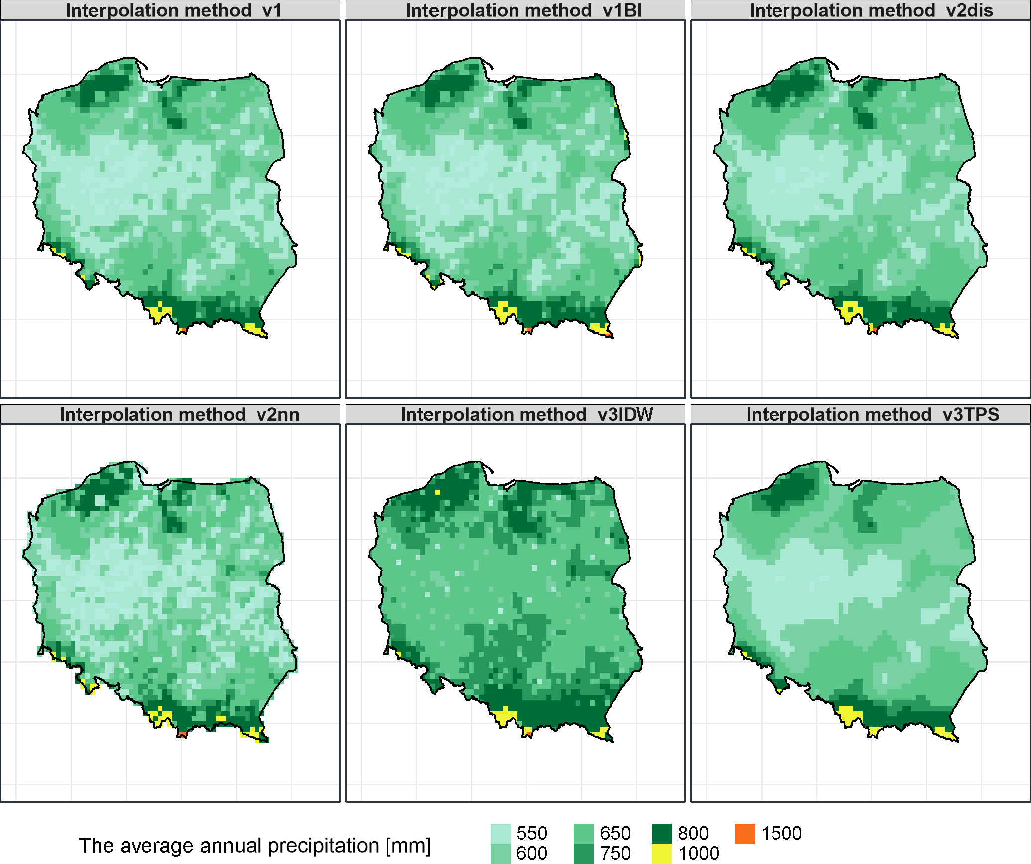
Analysis of these characteristics showed that the highest inconsistencies occurred for the v3IDW and v3TPS methods. For the v1BI method, there was an additional problem for three grid points located at the most southern end of the Polish border (Bieszczady National Park). For these three points, unrealistic values of the annual sum above 2600 mm were achieved (this is the maximum annual sum of precipitation for observational reference data), probably due to the extrapolation of data in the absence of a sufficient number of measurement points. As seen in Figure 3, for all methods except v3IDW, there is a middle band of lower annual precipitation totals and higher precipitation areas for the southern (mountain) and northern (coastal) extremes. For the v3IDW method, no such differentiation is apparent; the middle belt is not homogeneous (but it is impossible to distinguish), as is the case for other methods; and there are regular structures of lower and higher annual sums of precipitation. The remaining fields resemble the spatial distribution of annual rainfall totals for 2019 (IMGW-PIB 2020).
The analysis of the extreme values and the annual precipitation sum of percentiles provided a good result only for the maximum value. For the considered 120 stations, this value was 2600 mm, which occurred in 2001. All interpolation methods (for v1BI, the controversial three grid nodes were removed from the analysis) indicated the same year of occurrence and values ranging from 2097 mm to 2626 mm.
The variance inflation factor (VIF) was estimated for 96 stations for which time series of observations without missing data were available. The same stations were used in 4. Discussion for comparison of the resulting output methods of this work with data from the CHASE project (Berezowski et al. 2016; Piniewski et al. 2021). The results of the analysis are included in Table 4.
Table 4.
The variance inflation factor, the coefficient of determination, and the sum of squares of residuals for the mean annual sum of precipitation from 1976 to 2005.
The lowest variance inflation factor VIF (formula 2.5) was achieved for the v3IDW method (R 2 is the lowest for this method). For the IDW method on the analyzed sample, the sum of residuals was the highest, i.e., the sum of squares of the difference between observations and interpolated values. Results showed the lower the value of VIF and R2 (formula 2.6), the greater the SSres (formula 2.7) of the sum of squares of the difference of observations and interpolated values. A small variance of the interpolated values does not necessarily mean a good fit for the observational data.
3.2. Mean annual cycle of precipitation
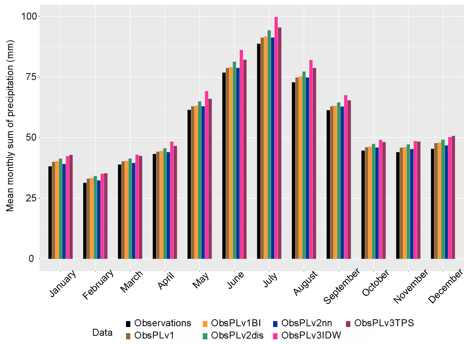
Based on the calculated 30-year average monthly sum of precipitation, the annual cycle of the monthly sum is presented in Figure 4. The overall assessment was positive for all models, and they all maintained the annual cycle. However, when calculating the percentage errors (in relation to the mean values for the observations) of the monthly averages, there was a division into two groups for better (methods v1, v1BI, v2nn) or worse (methods v2dis, v3IDW, v3TPS) reproduction of the annual cycle (Fig. 5). The lowest percentage error was achieved for the v2nn method for all months below 5%, and the highest for v3IDW for all months above 10%.

3.3. Monthly sum of precipitation
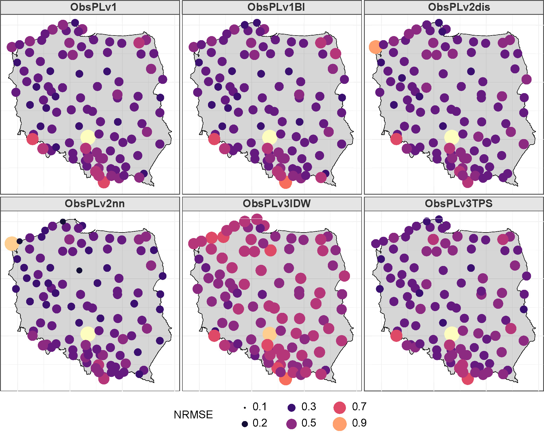
The analysis of the NRMSE and MAE values for the monthly precipitation sum is included in Table 5. The mean value of the NRMSE varied from 0.22 to 0.36, while the maximum value for all methods was at level 2. The mean value of MAE changed from 5.06 to 9.47. The large spread was reached by the maximum values of MAE from 30.8 to 48.3 mm, while the standard deviation SD of the MAE showed moderate variability ranging from 5.5 mm to ~8 mm. The NRMSE rating indicated the v2nn method, but the mean MAE exceeded 40 mm. The minimum value of the MAE was achieved by the v3IDW method, although this had the highest average error value.
Table 5.
Statistics for the error of the monthly sum of precipitation.
3.4. Maximum daily sum of precipitation in a month
A similar analysis was carried out for the maximum daily sum of precipitation. The mean value of the NRMSE (Fig. 6) ranged from 0.26 to 0.42. The mean value of MAE ranged from 1.78 to 2.82.
3.5. The 95th percentile of the daily total precipitation in a month
The maximum values depend on random outliers, but the reconstruction of the range of high daily total precipitation can be assessed based on the 95th percentile (Q95).
The assessment according to the Q95 parameter was more homogeneous for the interpolation methods (Table 6). The mean value of NRMSE varied from 0.40 to 0.48, the mean value of MAE did not exceed 2 mm, and the standard deviation SD of MAE changed from 1.89 to 2.27. Moreover, the lowest error parameters were achieved for the v3IDW method.
Table 6.
Statistics for the error of the 95th percentile of the daily total precipitation in a month.
3.6. The number of days with the daily sum of precipitation below 0.5 mm
Situations without precipitation or small daily total precipitation can be described using the number of days (LD05) in a month when the threshold was set to 5 mm.
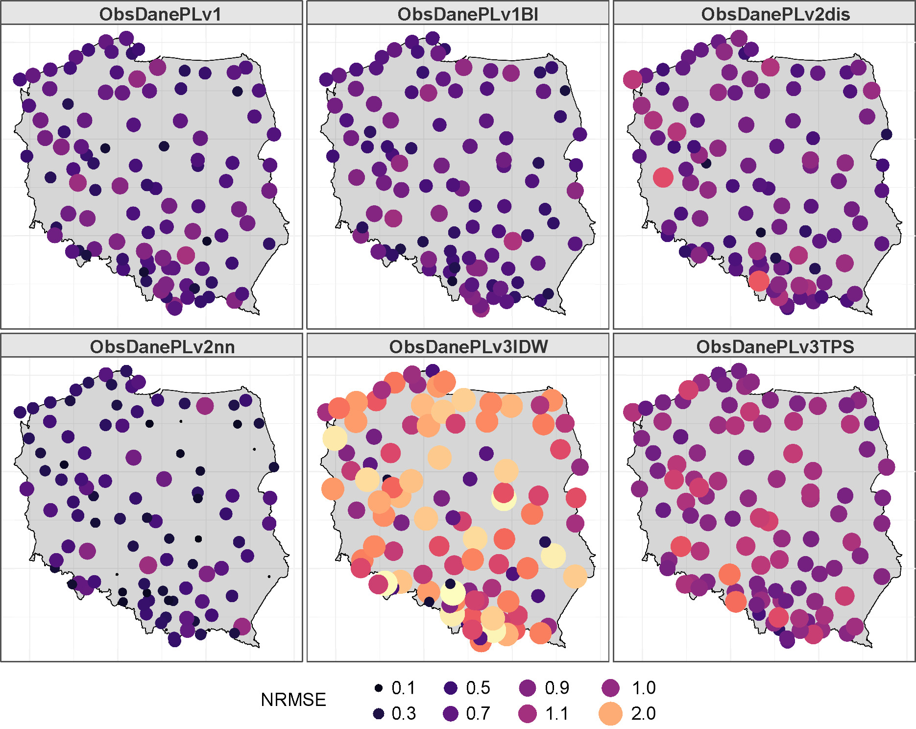
Table 7 presents the basic statistics of two commonly used metrics, NRMSE and MAE, for assessing the accuracy of an interpolated field of LD05. The table shows that v2nn had the lowest NRMSE (0.43) and the lowest MAE (1.22), suggesting it may be the most accurate method for interpolating the field. Conversely, v3IDW had the highest NRMSE (1.50) and the highest MAE (5.26), indicating that it may be the least accurate method. For the v3IDW and v3TPS methods, the value of NRMSE was greater than 1. This suggests that these methods may overestimate the number of days with precipitation. Additionally, the MAE’s standard deviation (SD) for these two methods was above 2, while it did not exceed 2 for the other methods. This indicates that the errors for v3IDW and v3TPS are more variable and less consistent than the errors for the other methods. Overall, these findings suggest that v3IDW and v3TPS may not be the most accurate methods for interpolating rainfall data in this context.
Table 7.
Statistics for the error of LD, the number of days in a month with a threshold of 5 mm.
Figure 7 illustrates that, with a few exceptions, the NRMSE for the v3IDW method was greater than that of the other methods throughout the entire domain.
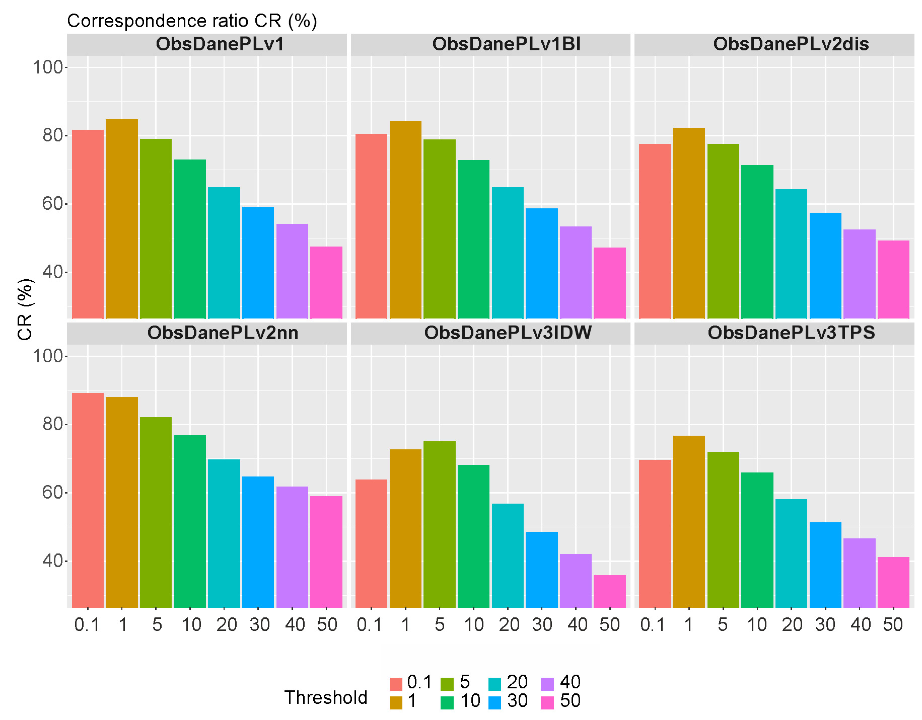
3.7. Correspondence ratio (CR) for the daily sum of precipitation
The CR measures the accuracy of spatial mapping by interpolation methods for areas with daily precipitation exceeding a threshold. The threshold of 0.1 mm indicates that even a small amount of fallout has been detected, which is referred to as a ‘trace’ amount. Certain areas were recreated correctly at 80% using different methods. However, two methods (v3IDW and v3TPS) did not perform as well as the others, achieving only 64% and 69% accuracy, respectively.
Figure 8 shows the analysis results for eight selected thresholds: 0.1, 1, 5, 10, 20, 30, 40, and 50 mm. The v2nn method achieved the best results, with close to 90% agreement for the 0.1 mm threshold and above 80% for the 1 mm threshold. For the 50 mm threshold, the agreement for the v2nn method is above 60%, while it ranges from 36% to 49% for the other methods.
3.8. Correlation coefficient (RO) for the daily sum of precipitation
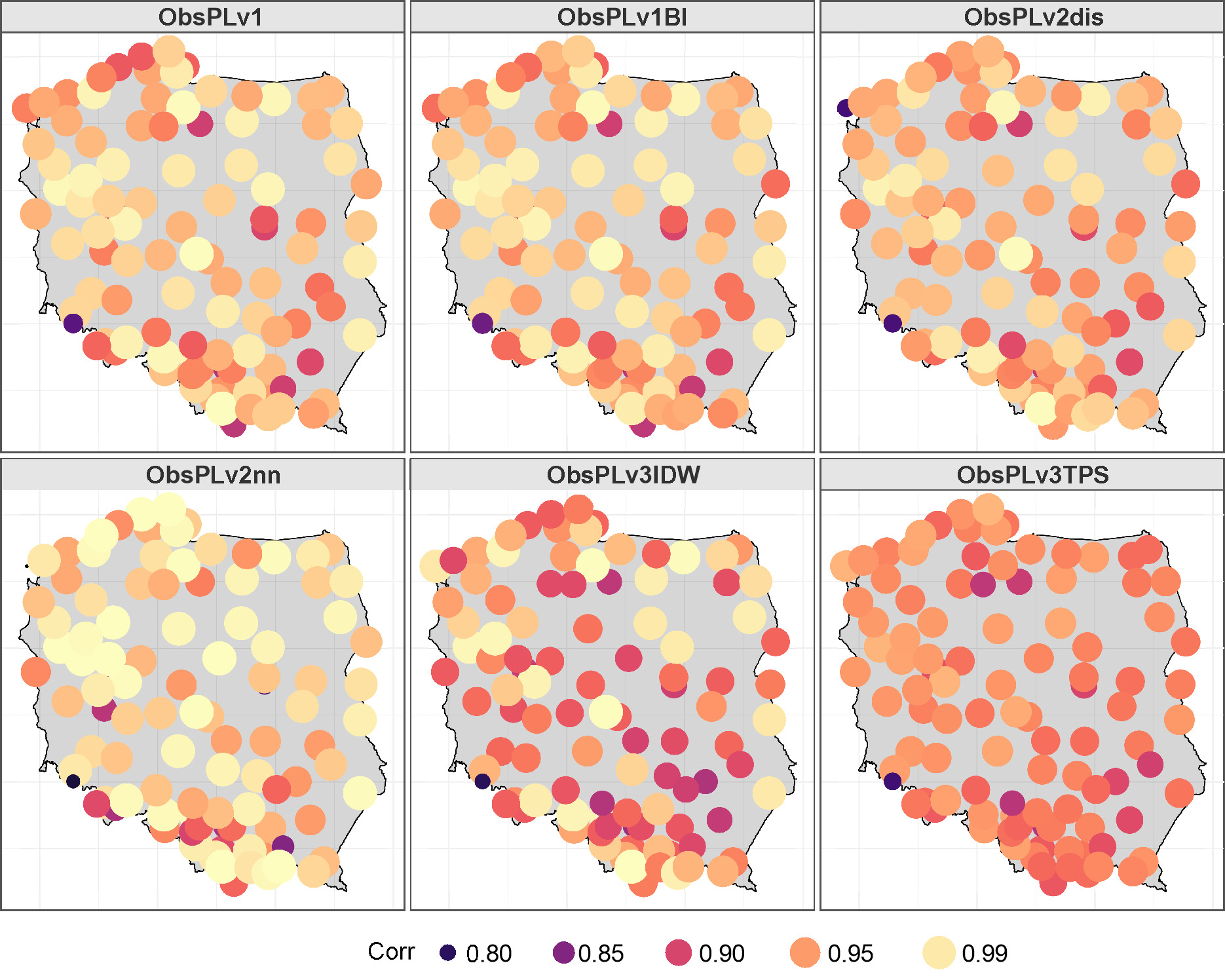
The RO value was analyzed in two ways. RO was calculated for the entire period, i.e., for the time series of interpolated values and observations. For all analyzed locations, the RO value was above 0.8, results are shown in Figure 9.
Fig. 9.
Map of the correlation coefficient of the daily sum of precipitation for the period 1976-2005.
In addition, the RO (the Pearson correlation coefficient) factor was calculated for individual days. In the absence of precipitation for more than 80% of observations, the RO was replaced with a measure of agreement in two–way tables. The basic characteristics calculated for these values indicated a slight differentiation when dividing the period into a warm and a cold half-year. For the warm half-year, the 25% RO quantile for the v3TPS method was 0.6; for the v2nn method, it was 0.9; and for the others, it was 0.8.
The median value of RO for this half-year was 0.9. For the cold half-year, the 25% quantile of the RO value for the v3TPS method was 0.6; for the remainder, it was 0.8. The median in the cold half-year for RO for the v3TPS method was 0.8, and for the other methods was 0.9.
3.9. Ranking of interpolation methods based on the average error
The calculated NRMSE/RSME and the MAE values allow ordering of the considered interpolation methods. A ranking of the methods was constructed considering these values for the maximum daily sum of precipitation in a month, the monthly sum of precipitation, the 95th percentile of the daily total precipitation, and the number of days with precipitation less than or equal to 0.5 in a month. The order of the methods in this ranking were v1, v2nn, v1BI, v2dis, v3IDW, and v3TPS (Table 8). There are six possible orders or rankings based on a certain parameter. Each number from 1 to 6 represents a different ranking, with 1 indicating the highest rank and 6 indicating the lowest rank.
Table 8.
Table of points for the ranking for NRMSE and MAE. Method
3.10. The resulting method for determining interpolated fields of daily precipitation totals
The choice of the reference field is essential because historical simulations show a differentiated fit to the field of observations, which translates into the selection and correction of climate scenarios and, thus, the conclusions resulting from the selected climate simulations.
None of the interpolation methods were outrightly superior. Most calculations indicated the v2nn method as the most appropriate interpolation method. However, the v2nn method failed when there was too little data around the node. There were unacceptable situations in the data for this method when interpolated monthly sums of precipitation in several nodes were zero for several years. Some interpolation methods overestimated the number of precipitation situations, and the resulting field of interpolated values was non-non-realistically smooth. However, such methods are irreplaceable in the case of missing observations when the alternative is the inability to perform the interpolation. The solution may be to select the interpolation method for individual days based on, for example, the CR and/or the RO value.
Analyses were performed for three datasets, in which the interpolation method was selected for each day. The adopted three selection criteria were based on the RO, the average correspondence ratio (CR_SR) for the thresholds of 0.1, 1, 5,10, and 20 mm, and based on both indicators together (RO_CR_SR). Three sets of complexes interpolated observational data RO, CR_SR, and RO_CR_SR were obtained by joining the appropriate fields interpolated for individual days. For the RO and CR_SR sets, the highest coefficient value on a given day determined the choice of the interpolation method. For the RO_CR_SR set, the interpolation method was selected based on rankings of the daily values of the RO and CR_SR parameters for the considered interpolation methods. Table 9 presents the statistics for each of the chosen interpolation methods.
Table 9.
Statistics (the correlation coefficient – RO, the average correspondence ratio – CR_SR, the correlation coefficient, and the average correspondence ratio – RO_CR_SR) for each chosen interpolation method for the sets of composite data from 1976-2005.
| Percentage of days for which the method was selected | ||||||
|---|---|---|---|---|---|---|
| Interpolated obs. | v1 | v1BI | v2dis | v2nn | v3IDW | v3TPS |
| RO | 11.7 | 13.4 | 8.6 | 47.0 | 14.1 | 5.2 |
| CR_SR | 7.7 | 5.8 | 4.8 | 72.7 | 3.6 | 5.4 |
| RO_CR_SR | 26.3 | 9.4 | 7.6 | 51.3 | 3.8 | 1.6 |
For each of the adopted criteria, the v2nn method – the nearest neighborhood – was chosen most often, in the case of the CR_SR criterion, as much as 72.7% of the time. For the datasets obtained in this way, an analysis of the fit was performed for the monthly sum (MS) of rainfall and the maximum rainfall in the month MAX for 102 stations.
For the MS of precipitation for all complex sets, the 75th percentile of NRMSE was below 0.3.
The maximum value for the NRMSE was greater than 1, but the value of NRSME=1.19 was only for one station (Czestochowa, 350190550), for the rest of this value is less than 0.76 (Table 10). The MAE statistics improved significantly, and the mean value was approximately 6 (previously ranging from 5 to 9.5). The maximum value of the MAE of approximately 50 mm was reached for the mountain station (Kasprowy Wierch, 1987 m above sea level). For the remaining analyzed stations, it did not exceed 27 mm.
Table 10.
Statistics (the correlation coefficient – RO_MS, the average correspondence ratio – CR_SR_MS, the correlation coefficient of the average correspondence ratio – RO_CR_SR_MS) for the monthly sum (MS) of precipitation in composite sets.
Table 11 contains statistics NRMSE and MAE for the maximum daily sum of monthly precipitation. The maximum NRMSE achieved for the Czestochowa station slightly exceeded 1; otherwise, this value was less than 0.71 (previously 1.78 to 2.82). The maximum values of MAE were around 11 mm, previously ranging from 8 to 12. The 75th percentile for MAE did not exceed 3 mm, and the median and mean values were around 2 mm.
Table 11.
Statistics of the fit error for the maximum daily sum of precipitation MAX for composite interpolation sets.
The average value of the CR for complex sets concerning individual interpolation methods was also analyzed. Figure 10 shows differences in the mean values of CR.
Fig. 10.
Differences in the mean correspondence ratio (CR) value for interpolation methods and complex sets RO, CR_SR, and RO_CR_SR. Rows refer to the complex sets RO, CR_SR, and RO_CR_SR. Columns correspond to the interpolation methods.
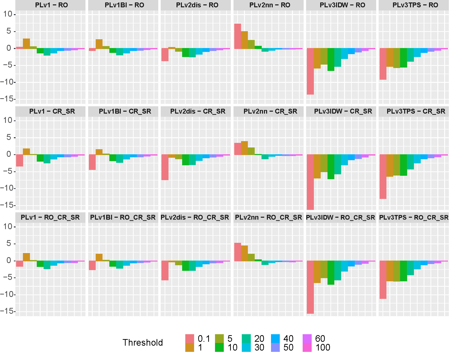
In most cases, the CR was greater for the sets RO, CR_SR, and RO_CR_SR than for individual interpolation methods. The exception was the nearest neighborhood method v2nn, for which the difference CR was positive for the thresholds 0.1, 1, 5, and 10. For the v3IDW and v3TPS methods, which were selected the least frequently in the result set according to the criteria based on RO and CR, the difference in the mean CR value was always negative. For the linear methods v1 and v1BI, the CR value was a few percent higher than for the complex sets only for the 1 mm threshold.
4. Discussion
The choice of the reference field is essential because the historical simulations show a differentiated fit to the field of observations. This translates into the selection and correction of climate scenarios, and thus, the conclusions resulting from the selected climate simulations.
The series of observational data differ in the amount and quality of data for each day of the period under consideration. In turn, interpolation methods react differently to this input data variability, and some are not disturbed by even a very small number of observations. As shown in the works cited (Sheffield et al. 2006; Prasad, Sushma 2016; Herrera et al. 2018; Crespi et al. 2019), these two factors significantly impact uncertainty in gridded precipitation datasets.
A comparative analysis using different statistical parameters for several selected interpolation methods for the entire period did not yield a ‘best method’. The v2nn method was chosen most frequently; but, for several years, for several nodes, the monthly sum of daily precipitation was zero. Other interpolation methods significantly overestimated the area of precipitation occurrence, inflated the extreme values, or the resulting field of interpolated values was non-non-realistically smooth. Correlation and correspondence ratio are important indicators of the quality of interpolated precipitation data, so a composite method based on both indicators was chosen. Three gridded datasets, RO, CR_SR, and RO_CR_SR, were prepared, in which the interpolation method was selected based on the values of the daily coefficients RO, CR, RO, and CR, respectively. The analysis comparing the monthly rainfall sums, the maximum daily sum in a month, and the correspondence ratio showed that the sets RO, CR_SR, and RO_CR_SR allowed for constructing more reliable data than the sets obtained using individual interpolation methods.
This approach allowed for the determination of gridded data based on different ways of selecting interpolation methods. Precipitation analysis concerns both the amount of precipitation and the area of occur-rence of this phenomenon, which can be described using indicators such as averaged CR and RO.
Interpolated precipitation data with a resolution of 5 km and 2 km (denoted as CHASE_5KM and CHASE_2KM, respectively) were provided in the CPLFD–GDPT5 (Berezowski et al. 2016) and G2DCPLC (Piniewski et al. 2021) projects. For selected locations, data from 1976-2005 were chosen and compared with analogous time series for datasets discussed in this paper (denoted as Comp_RO, Comp_CR_SR, and Comp_RO_CR_SR). The comparison was based on the MAE value for the annual sum of daily precipitation. The values of this error for all years and models ranged from 35.4 mm to 136.4 mm. The MAE values averaged over the period 1976-2005 are presented in Table 12.
Table 12.
Mean absolute error (MAE) for the annual sum of precipitation averaged over the period 1976-2005.
| Model | CHASE_2KM | CHASE_5KM | Comp_CR_SR | Comp_RO | Comp_RO_CR_SR |
|---|---|---|---|---|---|
| Mean of MAE | 99.4 | 106.0 | 49.1 | 53.3 | 50.1 |
The average MAE value for CHASE_2KM was 6.6 mm smaller than that for CHASE_5KM. The values for the ‘Comp’ group of models were approximately 50% lower than those for the ‘CHASE’ group. The comparison of the MAE for the annual sum of precipitation for each year of the period is presented in Figure 11.
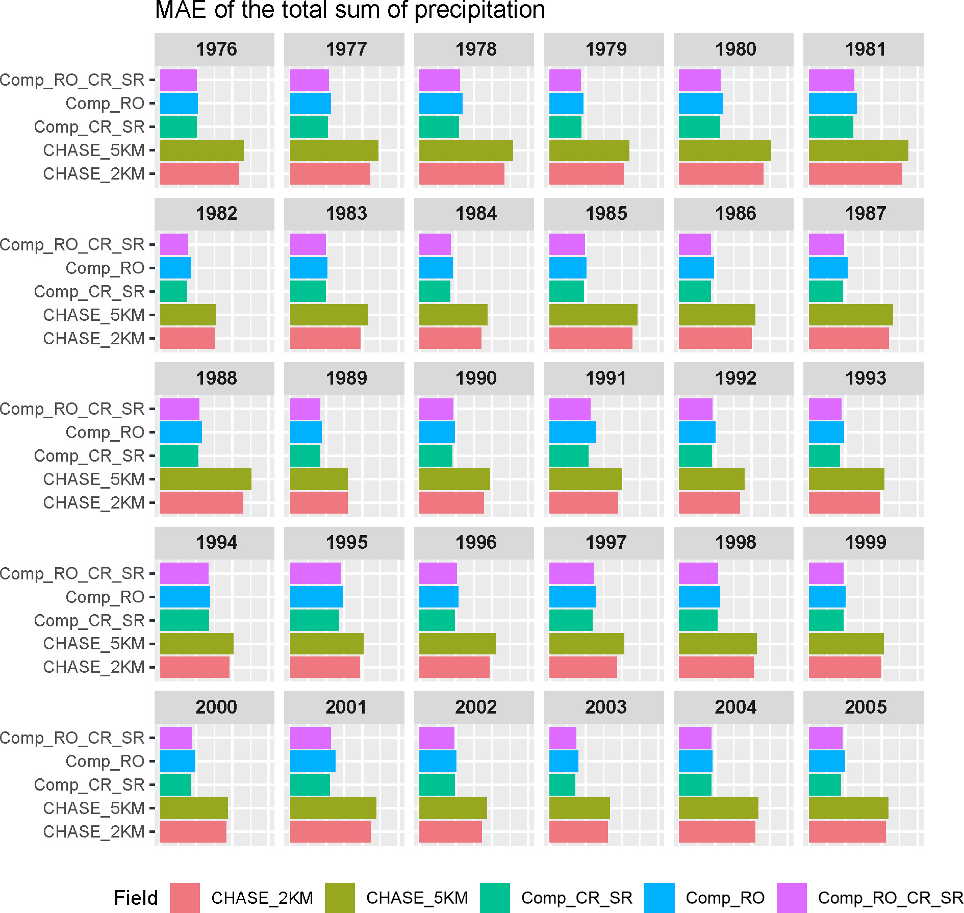
Figure 11 shows that for all years, the error for the ‘Comp’ models was smaller than that for the ‘CHASE’ models. This suggests that choosing more appropriate basic interpolation methods for each day, based on the values of the daily coefficients RO and CR, can significantly improve the resulting datasets.
The variance inflation factor of the average annual totals for compared fields was also analyzed (Table 13). The group of 96 stations was characterized by a high squared deviation from the mean, proportional to the variance value, SStot (2.8) was 3 203 554.
Table 13.
The variance inflation factor, the coefficient of determination, and the sum of squares of residuals for the mean annual sum of precipitation for resulting output methods of this work and data from the CHASE projects for 1976-2005.
As a result, the obtained VIF values ranged from 2.3 to 4.9, with values above 4.5 referring to the data obtained in this study. The application of the interpolated field selection method for individual days of the period resulted in the decrease of the VIF value below the value of 5.
5. Conclusions
This study introduced an innovative algorithm to determine the most appropriate interpolation method for each day based on the field fit characteristics at selected points. The selection procedure was based on the CR values (assessing compliance of areas with a given daily precipitation threshold) and /or RO (assessing the linear correlation). It was assumed that the potential uncertainty related to the different interpolation approaches used for each day would be compensated by greater compliance with rainfall areas and by maintaining a linear correlation. Among other things, the values of the variance inflation factor (VIF) were compared for the interpolation methods (Table 2), the three sets of complexes interpolated observational data (RO, CR_SR, and RO_CR_SR), and datasets CHASE from the CPLFD-GDPT5 (Berezowski et al., 2016) and G2DC-PLC (Piniewski et al. 2021) projects. The range of VIF values for the interpolation methods was from 3.2 to 6.3. For the sets of complexes interpolated observational data, VIF values were less than 5, which is lower than for most interpolation methods. For CHASE datasets, VIF was 2.3 for 5 km resolution and 2.9 for 2 km resolution. However, when comparing the latter two groups of datasets using the mean absolute error MAE, the average MAE error for the data resulting from this work was found to be 50% smaller. Our results provide evidence that expanding the range of available interpolation methods for each day and expanding the selection algorithm based on precipitation characteristics can significantly improve the resulting precipitation fields.