1. Introduction

In mountain catchments, climatic variables such as rainfall and temperature play a key role in hydrological processes such as runoff, evapotranspiration, and water yield prediction (Chiew, McMahon 2002; Chen et al. 2020; Kim, Kim 2020). Flood early warning and forecasting as well as drought management for mitigating water-related problems significantly rely on the accuracy of predicted spatial rainfall data input (Bertini et al. 2020; Lu et al. 2020).

Several scholars have provided basic information on the impacts of the spatial distribution of climatic variable input on further hydrological analysis and related problems. However, in developing countries such as Ethiopia, the spatial array of input climatic variable stations is sparse, and the density of climatological stations is extremely low (Washington et al. 2006; Dinku 2019). Therefore, the spatial interpolation method has been used to predict spatial values for unsampled points (Kim et al. 2010; Adhikary et al. 2017; Aydin 2018). This crucial method helps solve the issue of the sparse and low hydroclimatic network density and is widely used by governments and other sectors for planning water resource use and management at various spatiotemporal scales.

Spatial interpolation techniques require either ground-based observed climatic input data, radar rainfall, remote sensing-based satellite climatic input data, or blended data (Taesombat, Sriwongsitanon 2009; Verdin et al. 2015; Cantet 2017; Gebremedhin et al. 2021). The output of spatial interpolation is a map that shows the scale of the spatial climatic variable pattern of an area.

Digital elevation models (DEMs) are the main data commonly used as covariates in spatial interpolation techniques, specifically in geostatistics kriging. Several scholars have used topographic variables such as the elevation model as an explanatory variable and have confirmed that the covariate has a significant effect on the catchment’s hydrological system and water balance (Novikov 1981; Hudson, Wackernagel 1994; Vaze et al. 2010; Meena, Nachappa 2019). For instance, the elevation with different spatial resolutions brings a valuable change to the catchment’s spatial patterns of both rainfall and temperature (Hudson, Wackernagel 1994; Taesombat, Sriwongsitanon 2009). Research done by Taesombat and Sriwongsitanon (2009) revealed that the interpolation of point rainfall data using GLOBE-DEM (1000 m) and SRTM-DEM (90 m) elevation resolution as a predictor resulted in the coarser DEM resolution (GLOBE-DEM) performing slightly better in rainfall estimation than the finer one (SRTM-DEM). Vaze et al. (2010) investigated the effects of field survey DEM-derived elevation (25-m resolution) with finer-resolution light detection and ranging (LiDAR) DEM-derived elevation (1-m resolution) on the values of topographic indices, and the result showed that LiDAR DEM is a reasonably good representation of the real ground surface compared to DEMs derived from contour maps. Simanek and Holden (2020) suggest that DEM spatial resolution aggregated progressively to a coarser resolution, which resulted in decreased runoff and sediment.

Meena and Nachappa (2019) investigated the impacts of the DEM spatial resolution (12.5, 30, and 90 m) on landslide susceptibility mapping through a field survey, and the result depicted that the 30-m resolution is better suited for landslide susceptibility mapping. Numerous scholars have investigated the impacts of different spatial resolutions of DEM use on hydrological modeling (Schoorl et al. 2000; Wechsler 2007; Lin et al. 2010). For example, Lin et al. (2010) examined the effects of different DEM grid size resolutions on surface runoff and sedimentation using the SWAT model, and the results indicated that total phosphorous (TP) and total nitrogen (TN) decreased substantially with coarser resampled resolutions, whereas the predicted runoffs were not sensitive to resampled resolutions. The same result depicted the effect of grid size change on both the catchment landscape as well as the hydrological and geomorphic processes (Brown et al. 1993; Zhang, Montgomery 1994).

Although the Ethiopian landscape varies from flat to complex mountainous terrain, the impact of elevation horizontal resolution on rainfall and related climatological variable spatial distribution at the catchment scale is rarely considered and has not been extensively investigated. The studied catchment, Mille, has large topographic differences, with highly variable climatic and agro-ecological zones. Based on this, the objective of this study is to examine the effect of the DEM resolution on the spatial prediction of the catchment’s areal rainfall, maximum temperature, and minimum temperature, as well as to select the better and more reliable DEM resolution that serves as an auxiliary variable for future research work for the case of the Mille catchment in Ethiopia.

2. Study area

The studied catchment is located within the Awash River Basin (AwRB), which is the fourth largest basin in terms of area coverage and the seventh-largest basin in terms of surface water potential in Ethiopia (Berhanu et al. 2014). The Mille catchment area is nearly 5,599 km², situated to the east of the longest mountain chain of the western Awash River Basin escarpment encompassing the Mille River, which drains to the Awash River, between 11°17'-11°76'N latitude and 39°53'-40°94'E longitude. The topography of the Mille catchment ranges from steep mountainous terrain in the west to a gentle slope in the middle and undulating plains to the east (Fig. 1). The catchment elevations range from 412-755 m and 2,218-3,656 m above sea level for lowland plains and mountains, respectively. Land use/land cover is generally cultivated land, shrubland, woodland, forestland, grassland, bare land, and water bodies (MoWR 2009).

Fig. 1.

Location of the Mille catchment in Ethiopia.

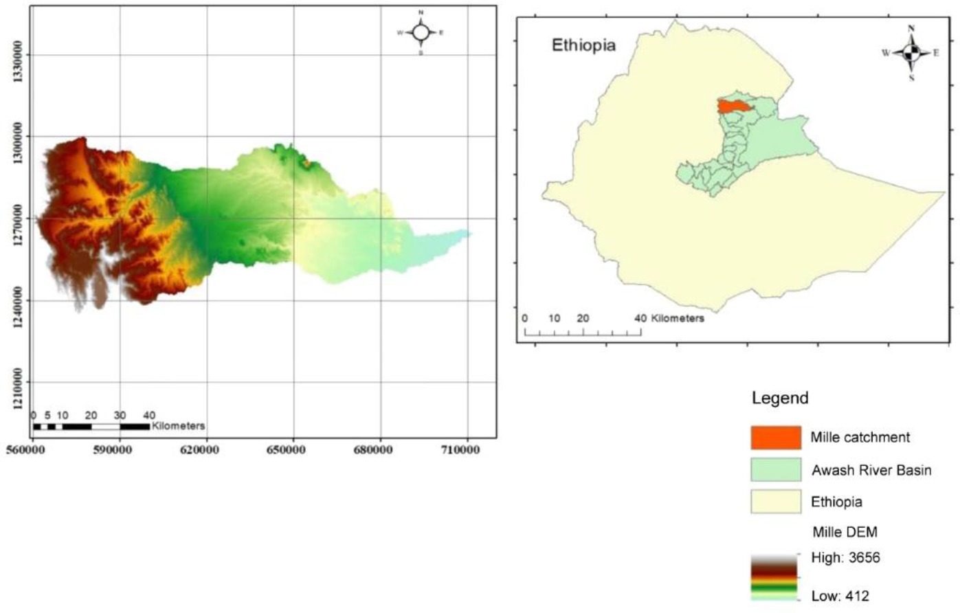
According to Berhanu et al. (2014), the catchment’s climatic zone falls within five agroclimatic zones of Ethiopia, ranging from hot arid (<500 m) in the east to humid (>3,200 m) near the remotest of the upper catchment. The annual rainfall pattern is bimodal (Berhanu et al. 2016), with rain occurring between June and August (main rainy season) and between March and May (pre-rainy season). Based on long-term historic climatic data (2000-2016), the estimated mean annual rainfall varies from approximately 465 mm on the easterly catchment to over 1,153 mm on the head of the drain catchment mountains, with a mean rainfall of 782 mm, and the estimated mean annual maximum and minimum temperatures vary between 29-43°C and 10-19°C, respectively.

2.1. Dataset

2.1.1. Rainfall and temperature data

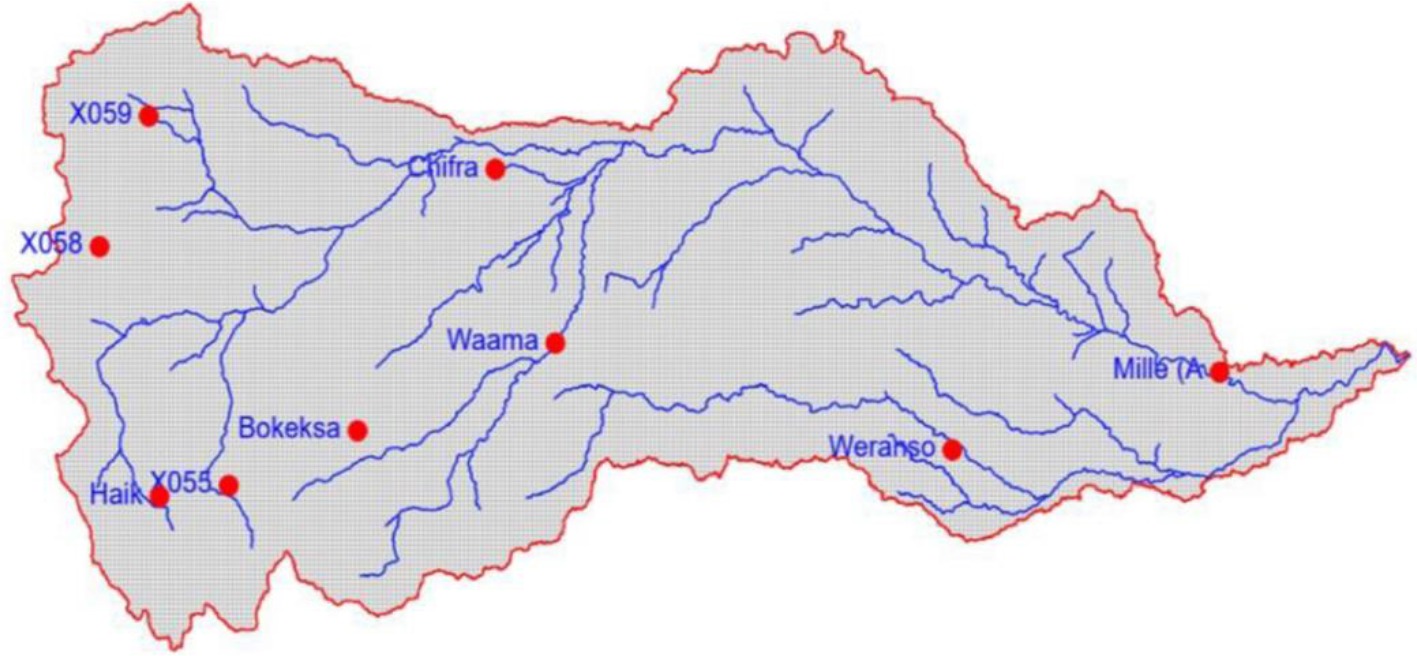
The rainfall and temperature datasets used in this study were provided by the Ethiopia National Meteorological Agency (ENMA). These datasets encompass mean monthly and annual rainfall and mean minimum and maximum temperature, which have completed, reliable, and useful historical samples masked from the long-term daily (2000-2016) national-level historic climate grid-based pixel dataset, as shown in Figure 2. These daily pixel datasets were blended by the project Enhancing National ClimaTe Services (ENACTS) at the national level, using combined satellite-based rainfall estimates and ground-based rainfall data for some African countries, such as Ethiopia; their consistency was checked using the double mass curve technique.

Fig. 2.

Mille catchment in Ethiopia and locations of sampled climate stations.

2.1.2. Digital elevation model (DEM) data

The Shuttle Radar Topography Mission (SRTM 3 arc-Second Global) digital elevation model (DEM) data were downloaded from NASA (https://urs.earthdata.nasa.gov) and resampled in steps to generate 500-m and 1,000-m DEMs. Resampling was done using the Resampling Technique parameter, Bilinear in Data management tools in ArcGIS. The study site DEM was extracted from each DEM spatial resolution, and these DEM resolution data, such as SRTM 90 m, SRTM 500 m, and SRTM 1000 m DEM, were used as a covariate in the analysis to investigate whether the spatial resolution of DEM data would have any impact on the accuracy of areal climatic variable interpolation.

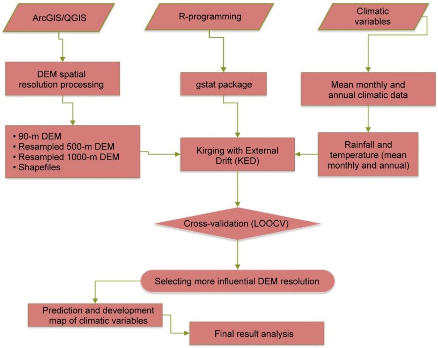
The spatial interpolation techniques were carried out by applying R programming used for the interpolation technique (Goovaerts 1997a) with the gstat package embedded within R (Pebesma, Wesseling 1998) to generate and evaluate the impacts of different resampled DEM spatial resolutions on climatological variable spatial prediction. The GIS tools (ArcGIS and QGIS) were used for processing DEM and preparing shapefiles.

2.2. Methods

Among the spatial interpolation techniques known as kriging (Matheron, Hasofer 1989), the geostatistical technique is considered the best unbiased linear predictor (BULP) for input data that satisfy the conditions of normality as the data are not skewed in any way (Isaaks, Srivastava 1994). However, climate data are often not symmetrical (skewness either to the right or to the left), which affects the spatial prediction of climate variables such as rainfall and temperature in that the few high values will overcome all the others. In experimental variogram prediction (Goovaerts 1997), nonsymmetric distributions are often transformed to conditions of normality using the natural logarithmic function and/or square root distance from the ocean/sea to minimize the skewness of input climate data and the influence of extreme values before variogram analysis and spatial interpolation (Goovaerts 1997). However, for small sampled data, such as our case, this can result in overprediction as well as empirical variograms that are difficult to model (Rossiter 2014). Therefore, the transformation was not applied because of the highly sparsely distributed climate data (see Fig. 2).

According to Goovaerts (1997), primary attributes of interest are usually accompanied by independent secondary information (auxiliary) that originates from continuous or random attributes, and the estimation generally improves when this information is taken into consideration, particularly in areas where the data are highly sparse or poorly correlated in space. Based on relevant literature reviews (e.g., Cantet 2017; Rata et al. 2020) and due to its high performance (in most cases) compared to other interpolation methods, kriging with external drift (KED) was selected to assess the effects of the catchment DEM spatial resolution on the spatial prediction of climatic variables. The methodological framework approaches used in this research article for the geostatistical interpolation technique were developed as follows (Fig. 3).

Fig. 3.

Schematic flowchart showing the estimation of spatial climatic variables.

2.2.1. Experimental Variogram

Of the sampled data, z(x₁), z(x₂) … z(x_n), where x₁, x₂, …, x_n represent the positions of the sampled in two-dimensional space, one can estimate both cloud and experimental variograms assuming those sampled data were unbiased.

The equation to compute the variogram is Matheron’s method of moments (MoM) estimator (Oliver, Webster 2015):

γ^(h)=12N(h)∑iN(h)z(xi)−z(xi+h)2, (1)

where γ^(h) is the experimental variogram, which equals one-half the squared difference between points separated by a distance x_i ± (x_i + h) (assuming no direction preference), z(x_i) and z(x_i + h) are the observed values of sampled data z at places x_i and x_i + h, and N(h)=N(N−1)2 is the number of paired values at lag h.

There are some methods to fit a variogram model to an experimental/empirical variogram, and this paper uses the exponential and spherical model (Eqs. 2 and 3) via a simple method called “automatic fitting variogram from the package automap.

γ(h)=c0+c{1−exp(−ha)},for 0 <  h0for h = 0  (2)

where c₀ is a nugget, c is the sill of variance, h is the lag, and a is the practical range.

γ(h)=c0+c3h2a−12ha3for 0 < h≤ ac0+cfor h > a0for h = 0  (3)

2.2.2. Kriging with an external drift

Kriging with an external drift (KED)¹ is a widely applied geostatistics interpolation method that considers auxiliary variables as external or secondary variables in the estimation of a primary attribute (Goovaerts 1997). In KED, a linear weighted average from the N known points with the value Z_i is used to estimate the value at each unknown point Z_o by using both the trend and local deviations (Rossiter 2019). The KED estimator is as follows:

Z^KED(X0)=∑i=1nλiKEDZ(Xi) (4)

Its expectation is as follows:

E[Z^KED(X0)]=∑k=0K ∑i=1nβkλiKED(Xi)  (5)

The estimator is unbiased if:

∑i=1nλiKEDYk(Xi) = Yk(X0)  (6)

3. Results

3.1. Effects of DEM spatial resolution on rainfall spatial prediction

The DEM elevations with various resolutions generated from the SRTM DEM covering the study area were between 490 and 2,088 m, 490.1 and 2,088.4 m, and 488.5 and 2,125.7 m above sea level (Table 1 and Fig. 4).

Table 1.

Elevation values for the nine sampled climatic stations.

Stations name	DEM's Elevation (m.a.s.l.)
	SRTM 90-m DEM	Resampled 500-m DEM	Resampled 1,000-m DEM
X055	2,088.0	2,088.4	2,125.7
X058	1,853.0	1,835.5	1,864.6
X059	1,574.0	1,566.0	1,559.0
Weranso	643.0	647.1	646.8
Waama	1,020.0	1,020.0	1,022.1
Mille (AVA)	490.0	490.1	488.5
Haik	2,003.0	1,996.9	2,012.8
Chifra	928.0	927.1	924.6
Bokeksa	1,768.0	1,733.3	1,747.2

Fig. 4.

Box plots of the descriptive statistical values of the elevations for nine sampled climatic stations.

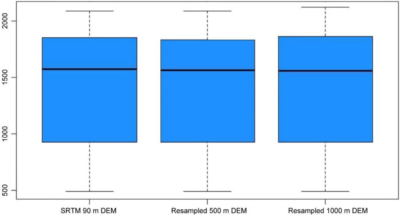
Table 1 shows that the maximum elevation value increased from 2,088 to 2,125.7 with coarsening DEM resolutions, and the minimum elevation value decreased from 490 to 488.5 as the DEM coarsened from 90 to 1,000 m. This may be due to the loss of detailed topographic attributes at coarser resolution (Zhang et al. 2014; Reddy 2015).

The spatial pattern mapped for mean monthly and annual rainfall was detailed with less error at the 500-m DEM resolution and the 90-m resolution than at the 1,000-m DEM resolution (Fig. 5 and Table 2). Based on the performance of the predicted rainfall values depicted in Table 2, the monthly rainfall data at each point were removed, and the remaining point input data were used to estimate the missing data by using the LOOCV procedure. Taking the rainy season (June, July, and August) into consideration, the KED technique with 500-m DEM as a covariate produced relatively smaller (larger in r) values of RMSE and MBE than the KED techniques with 90-m and 1,000-m DEM as a covariate for the spatial prediction of catchment rainfall both at monthly and annual temporal scales, respectively.

Fig. 5.

July and August mean monthly rainfall map for 17 years at (A) 500-m DEM resolution, (B) 1,000-m DEM resolution, and (C) 90-m DEM resolution using KED.

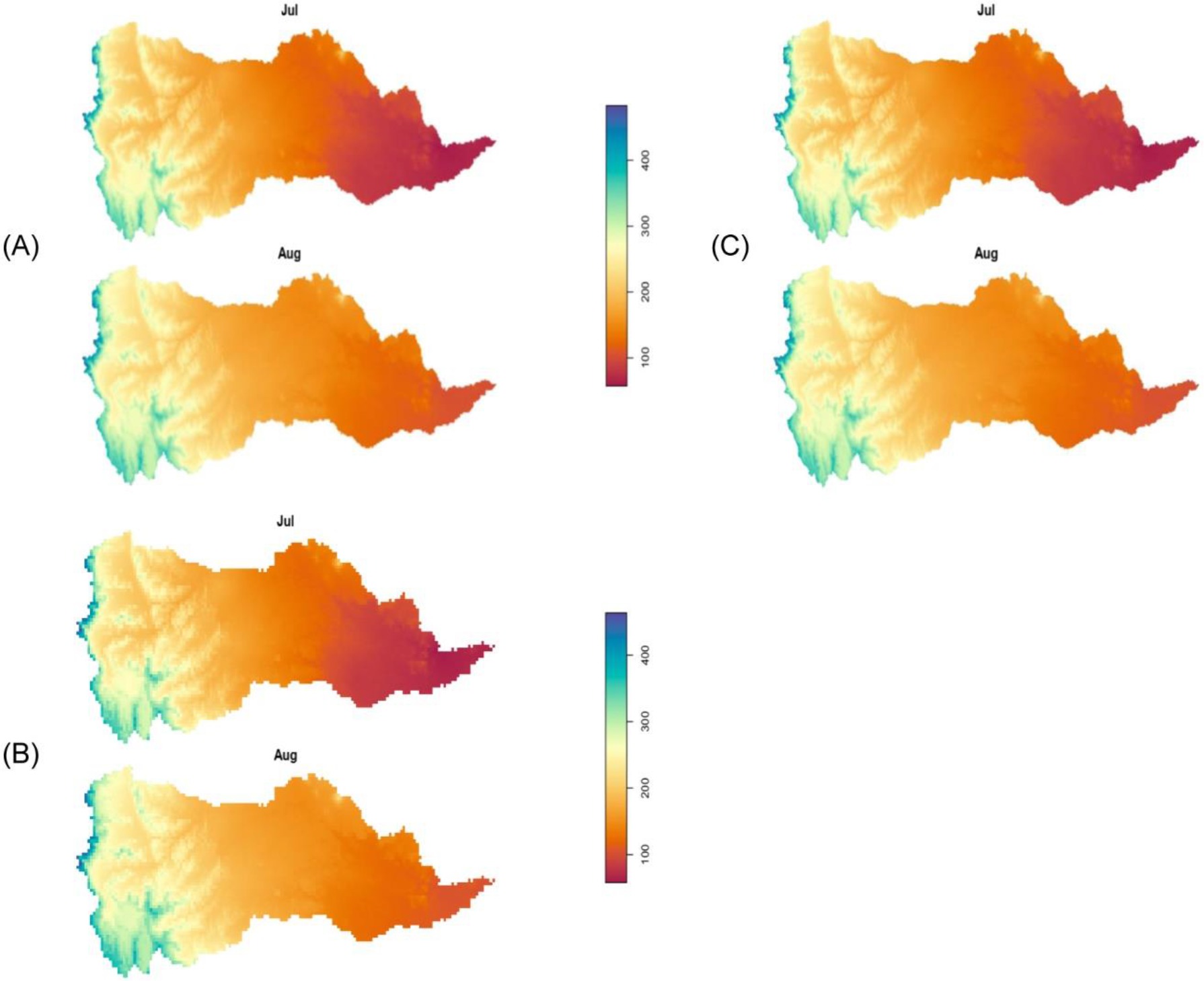
Table 2.

Statistical evaluation of the impact of DEM resolution on spatial rainfall prediction.

Month	Ro	90-m DEM and evaluation criteria				500-m DEM and evaluation criteria				1,000-m DEM and evaluation criteria
		Re	RMSE	MBE	r	Re	RMSE	MBE	r	Re	RMSE	MBE	r
Jan	11.42	11.79	5.72	–0.36	–0.015	11.82	5.77	–0.39	–0.047	11.83	5.81	–0.4	–0.067
Feb	6.799	6.752	3.17	0.05	0.570	6.748	3.14	0.05	0.578	6.758	3.16	0.04	0.572
Mar	37.92	38.33	9.05	–0.41	0.856	38.32	9.00	–0.41	0.858	38.36	9.27	–0.45	0.848
Apr	57.64	58.13	9.91	–0.49	0.863	58.15	10.00	–0.51	0.860	58.19	10.33	–0.55	0.850
May	43.40	43.95	9.26	–0.56	0.838	43.96	9.32	–0.57	0.835	44.01	9.63	–0.61	0.824
Jun	16.49	16.617	4.35	–0.13	0.878	16.616	4.32	–0.13	0.880	16.638	4.44	–0.15	0.873
Jul	192.76	194.87	35.96	–2.11	0.891	194.86	35.64	–2.10	0.893	194.92	36.08	–2.16	0.890
Aug	216.06	218.1	34.81	–2.05	0.878	218.1	34.24	–2.03	0.882	218.2	35.09	–2.13	0.875
Sep	64.03	64.69	13.45	–0.67	0.871	64.73	13.68	–0.70	0.866	64.79	14.12	–0.76	0.857
Oct	24.16	24.64	7.39	–0.48	0.746	24.66	7.46	–0.50	0.741	24.68	7.60	–0.52	0.730
Nov	16.08	16.25	2.76	–0.17	0.849	16.25	2.75	–0.17	0.851	16.26	2.81	–0.17	0.844
Dec	12.00	12.232	4.71	–0.24	0.500	12.243	4.74	–0.25	0.490	12.253	4.80	–0.26	0.475
Annual	698.8	706.4	123.96	–7.64	0.884	706.8	122.65	–7.52	0.894	706.8	127.35	–8.08	0.877

[i] NB: R_o = observed mean rainfall (mm), R_e = estimated mean rainfall (mm).

On the other hand, the rainfall spatial distribution in two months, such as December and February, was less correlated with an auxiliary variable (elevation) and its resolution. Surprisingly, January’s monthly spatial rainfall distribution was exceptional and was less negatively correlated with elevation itself and its resolution. The reasons were that supplements to local factors (e.g., topography), the spatial rainfall patterns were affected by different global and regional factors, such as the Inter-Tropical Convergence Zone (ITCZ), Tropical Easterlies, interseasonal variation, and latitudinal locations (Dawit 2010; Melesse et al. 2014). The results indicate that the KED with the 500-m DEM as a covariate was the most suitable for mean monthly and annual areal rainfall estimation compared to the other DEM resolutions.

In general, the point rainfall depths vary with spatial and temporal scales and tend to increase with increasing elevations because of the orographic effect, which results in a lifting of air vertically and forms clouds due to the adiabatic cooling effect.

3.2. Effects of DEM resolution on the spatial pattern of temperature

The spatial map of maximum temperature produced by KED using various DEM resolutions as a covariate showed more gradual and smoothing changes, with a regular distribution in the middle to the lower parts of the catchment. At the uppermost and escarpment parts of the catchment, the spatial map appeared irregularly distributed and with discontinuous borders, showing an abrupt change in spatial distribution (Fig. 6A-C).

Fig. 6.

May and June mean monthly maximum temperature map for 17 years at (A) SRTM 90-m DEM resolution, (B) SRTM 1,000-m DEM resolution, and (C) SRTM 500-m DEM resolution using KED.

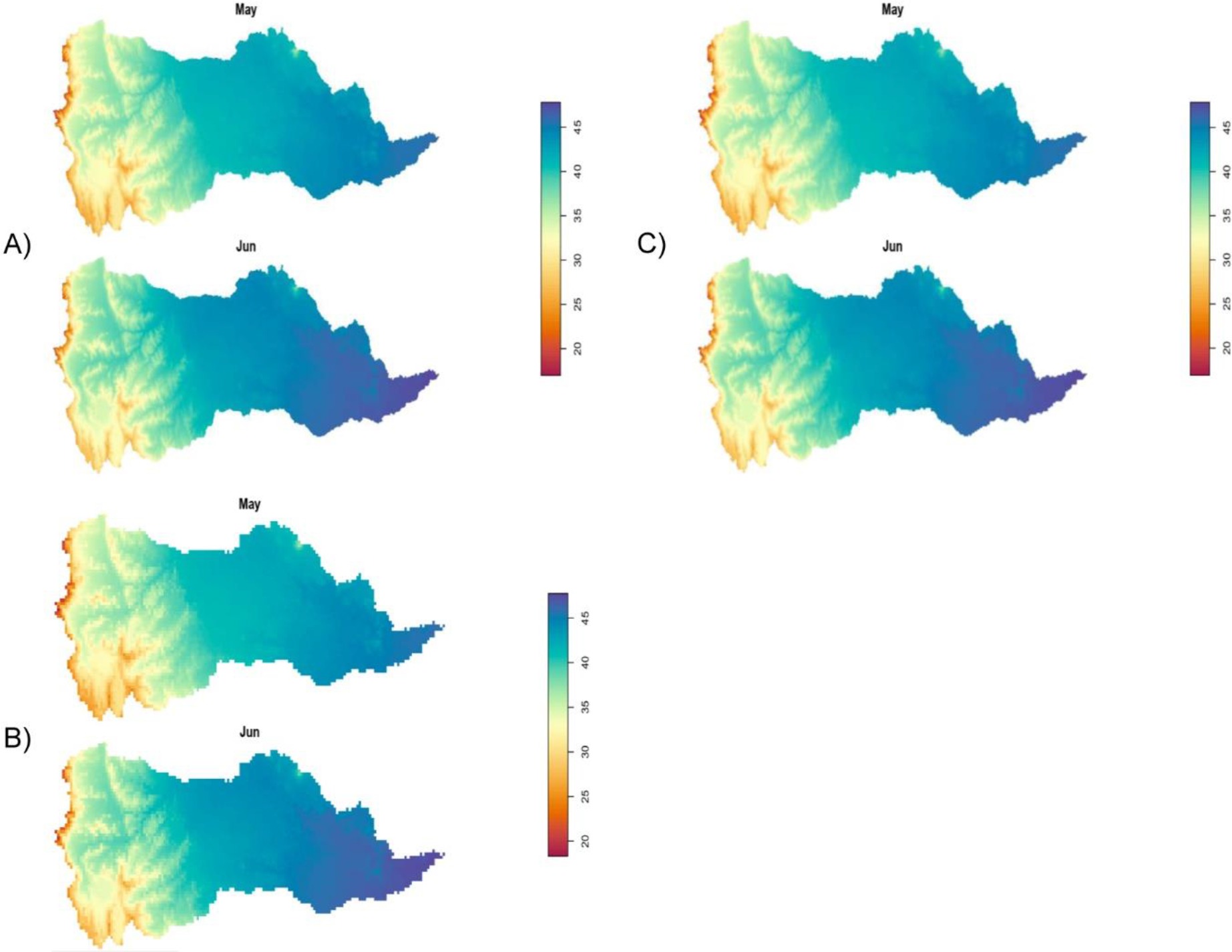
Tables 3 and 4 show that the spatially predicted mean maximum and minimum temperature values were similar to the analyzed predicted rainfall in that they were significantly influenced by the DEM but less influenced by the DEM’s horizontal resolution. Based on the statistical evaluation of three DEM resolutions in terms of RMSE, MBE, and r of the KED technique, the 90-m DEM resolution depicted the lowest error (highest r value) relative to the remaining DEM resolutions on maximum and minimum temperatures. As depicted in Figure 6A-C, the spatial pattern of maximum temperature gradually increases from west to the east following the elevation, which decreases progressively from west to east. Thus, based on the visual inspection of expert knowledge and statistical evaluations, it can be concluded that the spatial distributions of the mean minimum and maximum temperatures were presented in better detail at a 90-m DEM resolution than at the other DEM resolutions.

Table 3.

Mean monthly and annual maximum values observed and estimated temperature (°C) and covariates.

Month	(Tmax)o	SRTM 90-m DEM and evaluation criteria				SRTM 500-m DEM and evaluation criteria				SRTM 1,000-m DEM and evaluation criteria
		(Tmax)e	RMSE	MBE	r	(Tmax)e	RMSE	MBE	r	(Tmax)e	RMSE	MBE	r
Jan	31.62	31.71	1.73	–0.09	0.897	31.70	1.77	–0.08	0.892	31.70	1.76	–0.07	0.893
Feb	33.47	31.71	0.68	0.02	0.984	33.45	0.73	0.02	0.981	33.45	0.76	0.03	0.980
Mar	36.06	36.11	1.69	–0.05	0.938	36.10	1.74	–0.04	0.935	36.10	1.71	–0.03	0.936
Apr	36.69	36.77	1.45	–0.08	0.966	36.76	1.52	–0.07	0.963	36.75	1.50	–0.07	0.964
May	37.36	37.38	0.90	–0.02	0.985	37.38	0.97	–0.02	0.983	37.37	0.98	–0.01	0.982
Jun	39.01	39.08	1.89	–0.07	0.941	39.07	1.97	–0.05	0.935	39.05	1.97	–0.04	0.935
Jul	38.86	38.99	2.20	–0.14	0.933	38.99	2.27	–0.13	0.929	38.98	2.27	–0.12	0.929
Aug	35.77	35.85	1.43	–0.08	0.974	35.84	1.49	–0.07	0.972	35.84	1.47	–0.06	0.973
Sep	34.38	34.32	1.64	0.06	0.960	34.31	1.68	0.06	0.958	34.31	1.70	0.07	0.957
Oct	34.33	34.36	1.16	–0.03	0.979	34.36	1.23	–0.03	0.976	34.35	1.24	–0.02	0.975
Nov	33.04	33.18	2.14	–0.14	0.916	33.17	2.20	–0.13	0.912	33.16	2.16	–0.12	0.914
Dec	30.42	30.43	0.62	–0.02	0.987	30.43	0.67	–0.02	0.985	30.43	0.68	–0.01	0.985
Annual	35.08	35.13	1.17	–0.05	0.974	35.13	1.23	–0.05	0.971	35.12	1.22	–0.04	0.971

[i] NB: – (T_max)o – observed mean maximum temperature, (T_max)e – estimated mean maximum temperature.

Table 4.

Mean monthly and annual minimum values observed and estimated temperature (°C) and covariates.

Month	(Tmin)o	SRTM 90-m DEM and evaluation criteria				SRTM 500-m DEM and evaluation criteria				SRTM 1,000-m DEM and evaluation criteria
		(Tmin)e	RMSE	MBE	r	(Tmin)e	RMSE	MBE	r	(Tmin)e	RMSE	MBE	r
Jan	11.63	11.569	0.88	0.06	0.945	11.569	0.86	0.06	0.947	11.567	0.88	0.06	0.945
Feb	12.46	12.381	1.10	0.08	0.941	12.381	1.09	0.08	0.942	12.379	1.12	0.08	0.939
Mar	14.00	13.930	0.98	0.06	0.951	13.910	1.00	0.07	0.948	13.890	1.02	0.07	0.946
Apr	15.64	15.580	0.89	0.06	0.965	15.580	0.92	0.06	0.962	15.570	0.94	0.06	0.960
May	16.71	16.630	0.97	0.06	0.968	16.640	0.97	0.07	0.968	16.620	1.01	0.07	0.966
Jun	17.68	17.600	1.17	0.08	0.966	17.600	1.18	0.08	0.965	17.610	1.22	0.08	0.963
Jul	17.47	17.410	0.95	0.06	0.969	17.410	1.00	0.07	0.966	17.400	1.02	0.07	0.965
Aug	16.41	16.340	1.09	0.07	0.950	16.330	1.12	0.07	0.947	16.330	1.14	0.08	0.945
Sep	16.00	15.920	1.23	0.08	0.950	15.920	1.24	0.08	0.948	15.910	1.28	0.08	0.946
Oct	13.24	13.165	1.07	0.08	0.958	13.166	1.06	0.07	0.960	13.163	1.09	0.08	0.957
Nov	11.49	11.404	1.40	0.09	0.909	11.404	1.37	0.09	0.913	11.402	1.38	0.09	0.911
Dec	10.71	10.641	1.04	0.07	0.936	10.641	1.01	0.07	0.939	10.640	1.02	0.07	0.937
Annual	14.46	14.389	1.03	0.07	0.956	14.390	1.02	0.07	0.957	14.388	1.04	0.07	0.955

[i] NB: – (T_min)o – observed mean minimum temperature, (T_min)e – estimated mean minimum temperature.

4. Discussion

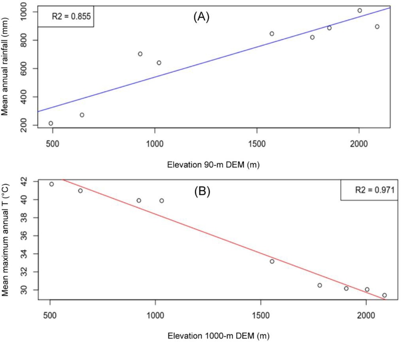
As illustrated in Figures 7A and B, the relationships between the mean annual rainfall and the mean maximum annual temperature of each sampled climatic station between 2000 and 2016 and its elevation were plotted. The mean annual rainfall and mean maximum annual temperatures tended to increase/decrease with increasing observed elevations, with coefficients of determination of 0.86 and 0.97, respectively. However, the spatial resolution among the three DEMs had no significant effect on the spatial prediction of climatic variables (see Tables 2 and 3). The analysis indicates that the most important characteristics, such as the mean annual and mean monthly climatological variables, rainfall and temperature, were significantly correlated with DEM elevation but less correlated with DEM resolution.

Fig. 7.

Correlation diagram of annual mean predicted rainfall (A) and mean maximum predicted temperature (B) with elevation.

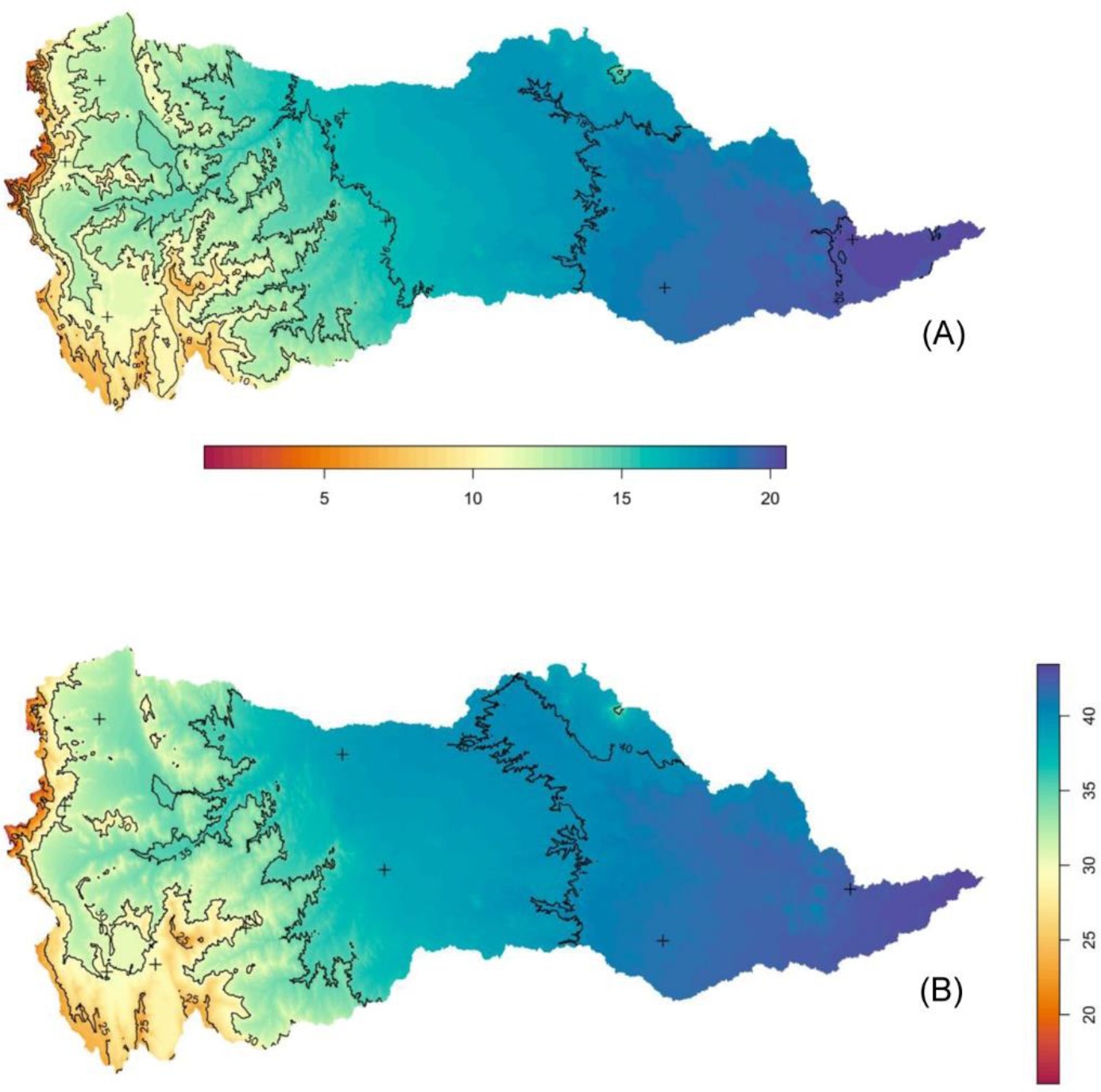
The predicted minimum and maximum temperatures were interpolated and extrapolated by KED to unsampled regions with a well-performing horizontal resolution DEM as a covariate (Figs. 8A, B). As seen in the developed maps, the highest amounts of spatial temperature were distributed in the catchment at the lowest elevations, which confirms that the spatial distribution of mean temperature is linearly correlated with the selected DEM (see Tables 3 and 4).

Fig. 8.

Spatial map of the mean minimum and maximum annual temperatures with 90-m elevation as external drift, using the sampled stations.

The primary novelty of the study resides in the evaluation and selection of DEM with the spatial resolution which shows relatively good performance in the prediction of the spatial distribution of climatological variables based on cross-validation techniques and, to some extent, expert knowledge. According to the proposed techniques, selecting covariates slightly improves the predictive performance of KED. For instance, the mean annual rainfall predicted using elevation with spatial resolutions of 500 and 90 m showed a slightly good performance (RMSE = 122.65, MBE = –7.52, r = 0.89, and RMSE = 123.96, MBE = –7.64, r = 0.88) r compared to the 1,000-m resolution DEM (RMSE = 127.35, MBE = –8.08, r = 0.877).

The proposed procedure achieved good performance regarding the prediction of mean minimum and maximum annual and monthly temperature with elevation but showed lower performance on the prediction of both mean monthly and annual temperature with various DEM resolutions. Similar to a previous study (Taesombat, Sriwongsitanon 2009), the optimum coarser DEM (500-m SRTM-DEM) resolution seemed to outperform both the mean monthly and annual rainfall estimations compared to the finer DEM (90-m SRTM-DEM) and coarser (1,000-m SRTM-DEM) resolutions, whereas the fine resolution (90-m SRTMDEM) showed relatively less error in the mean monthly minimum and maximum temperature estimations than the remaining two DEM resolutions. This approach seems to be a great opportunity to perform and select the more advanced horizontal resolution of DEM, which is used as a predictor for geostatistical interpolation techniques in mountainous catchments with overly sparse and unrepresentative observational climatic data.

5. Conclusions

This study compared and examined the impacts of three DEM resolutions (SRTM 90-m DEM, SRTM 500-m DEM, and SRTM 1,000-m DEM) on the spatial prediction of rainfall and temperature in a topographic complex catchment by using the KED interpolation technique. Three different DEM resolutions were tested on a 5599-km² catchment. The minimum and maximum elevations in the catchment varied substantially due to DEM resolutions (see Table 1), and the results indicated that changes in DEM resolution somehow influenced the outcomes of the prediction performance for both rainfall and temperature. In general, there were two different effects of DEM resolution. The first was the overestimation of mean monthly and annual rainfall and maximum temperature, and the second was the underestimation of mean monthly and annual minimum temperature. The LOOCV procedure infers that for mean monthly and annual rainfall, the coarser DEM resolution (500-m SRTM-DEM) performed better in spatial prediction with less error, whereas for mean maximum and minimum temperature spatial estimation, the finer DEM resolution (SRTM 90-m DEM) performed slightly better than the remaining DEM spatial resolution. This type of interpolation technique plays a fundamental role in various applications by assessing the effects of climate on hydrology, the environment, agricultural activities, and water resource development. Overall, the findings in this paper confirm that, as the DEM resolutions vary, the impact on the spatial prediction of the climatic variable is less significant. However, a substantial difference in resolution brings a small elevation change (vertical height), and this may affect hydrologically important topographic attributes calculated from DEM, such as slope, aspects, and drainage networks, specifically in mountainous catchments (Wilson et al. 1998). There are important implications for those interested in using spatially distributed topographic attributes for further applications (Moore et al. 1991; Brown et al. 1993; Lin et al. 2010). Therefore, it is recommended to consider further application uses, specifically in mountainous catchments.