1. Introduction

In recent years the hydrological cycle has been escalating and hastening because of climate change, with consequences that include increasing frequency and magnitude of floods (Kvočka et al. 2015). Floods are the most common and extreme catastrophes in a tropical country like India. Floods cannot be completely avoided, but the accompanying threats could be minimized, if flood prone areas are known in advance (Sahoo, Sreeja 2015). Therefore, recognizing flood risk zones and flood inundation mapping (FIM) are key steps for framing flood management strategies (Sahoo, Sreeja 2015). Correct geometry and flow data inputs are basic requirements of a good hydraulic model, but the performance of the simulations also varies by model type, e.g., one dimensional (1-D), two dimensional (2-D) or combined (1-D & 2-D) types. 1-D models are used extensively to simulate flow in the main river channel and in certain cases very effective in predicting flood extent (Vozinaki et al. 2016). Computational effectiveness and simple parameterization in dealing with flows in large and complex networks have been established by 1-D modelling (Ahmad, Hassan 2011). Horritt and Bates (2002) checked performance of 1-D modelling for hydraulic simulation by carrying out numerous studies and concluded that 1-D models have sufficient skill for good estimation of flood level and flood travel time, so that it can be used for prediction of flood extent. Timbadiya et al. (2012) developed a calibrated HEC-RAS-based model using flood peaks of observed and simulated floods; root mean squared error (RMSE) demonstrated that predicted flood levels were satisfactory. In the present study, a 1-D hydrodynamic model has been developed by using the Hydrologic Engineering Center’s River Analysis System (HEC-RAS, V. 5.0.7) developed by the U.S. Army Corps of Engineers (USACE).

2. Governing equations

where: Q – discharge [m³/sec]; A – cross-sectional area [m²]; g – acceleration due to gravity [m/sec²]; β – momentum correction factor; h – elevation of the water surface(stage) in meters above a specified datum; s_o – bed slope (Longitudinal channel bottom slope); t – temporal coordinate; x – longitudinal coordinate.

3. Numerical solution methods

Numerical techniques for the solution of expanded Saint-Venant equations can be given by implicit finite difference techniques with the most widely used Preissmann technique. In this technique all derivative terms and other parameters are calculated by using unknowns at the forward timeline (j+1) in x-t grid as shown below.

Fig. 1.

The distance-time grid to developed implicit finite difference scheme.

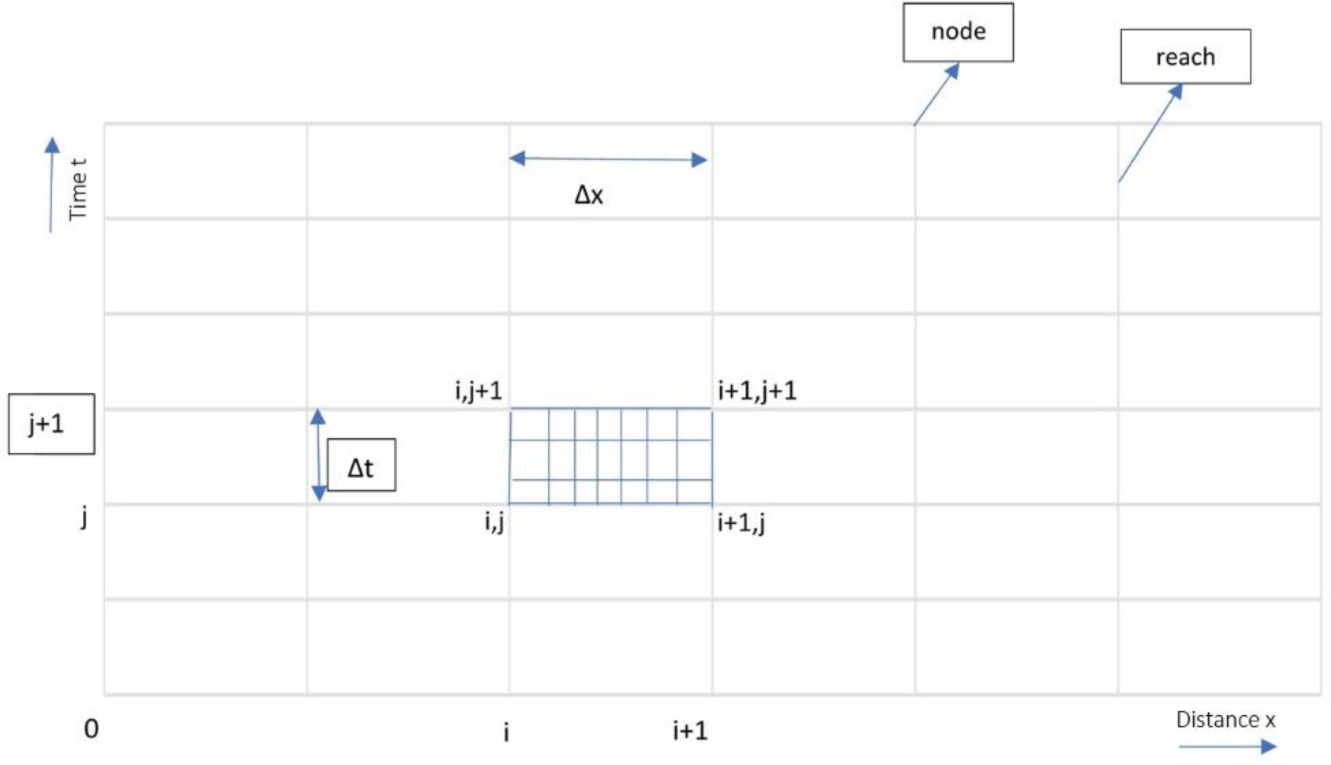
In this scheme, grid size is taken as (i, j) where: i is the space interval; j is the time interval, and the four grid points from the (j)^th and (j+1)^th timelines are taken to approximate for the differential equation. A weighing factor, (θ = 0.5) is used in the approximation of all terms of the equation except for the time derivatives in order to adjust the influence of the points (i) and (i+1). Partial differential equations of continuity and momentum are obtained as a result of approximation by the Preissmann implicit finite difference scheme.

Water level (h) = f(A,B), where A is the cross-sectional area; B is the channel top width

Where hNj+1 is the stage to be computed at downstream and h(t) is the stage hydrograph value input to the model.

Discharge, water level, and area of cross-section are stated at nodes of grid and S_o, S_f, S_e i.e. bed slope, friction slope and energy line slope are stated at reaches.

Space derivatives of the Saint-Venant equations are:

Time derivatives of the Saint-Venant equations are:

Other factors, A, Sf, q are approximated as follows:

Substituting all values into the continuity equation yields,

Putting all values into the momentum equation yields,

These equations are solved by the Newton-Raphson iterative technique to calculate water level and discharge at (j+1)^th timeline at nodes (i) and (i+1).

4. Methodology adopted

A hypothetical, rectangular river section was established, assuming a width of 800 m, an average longitudinal bed slope of 0.0005, and Manning’s roughness coefficient of bed slope changing with time and distance.

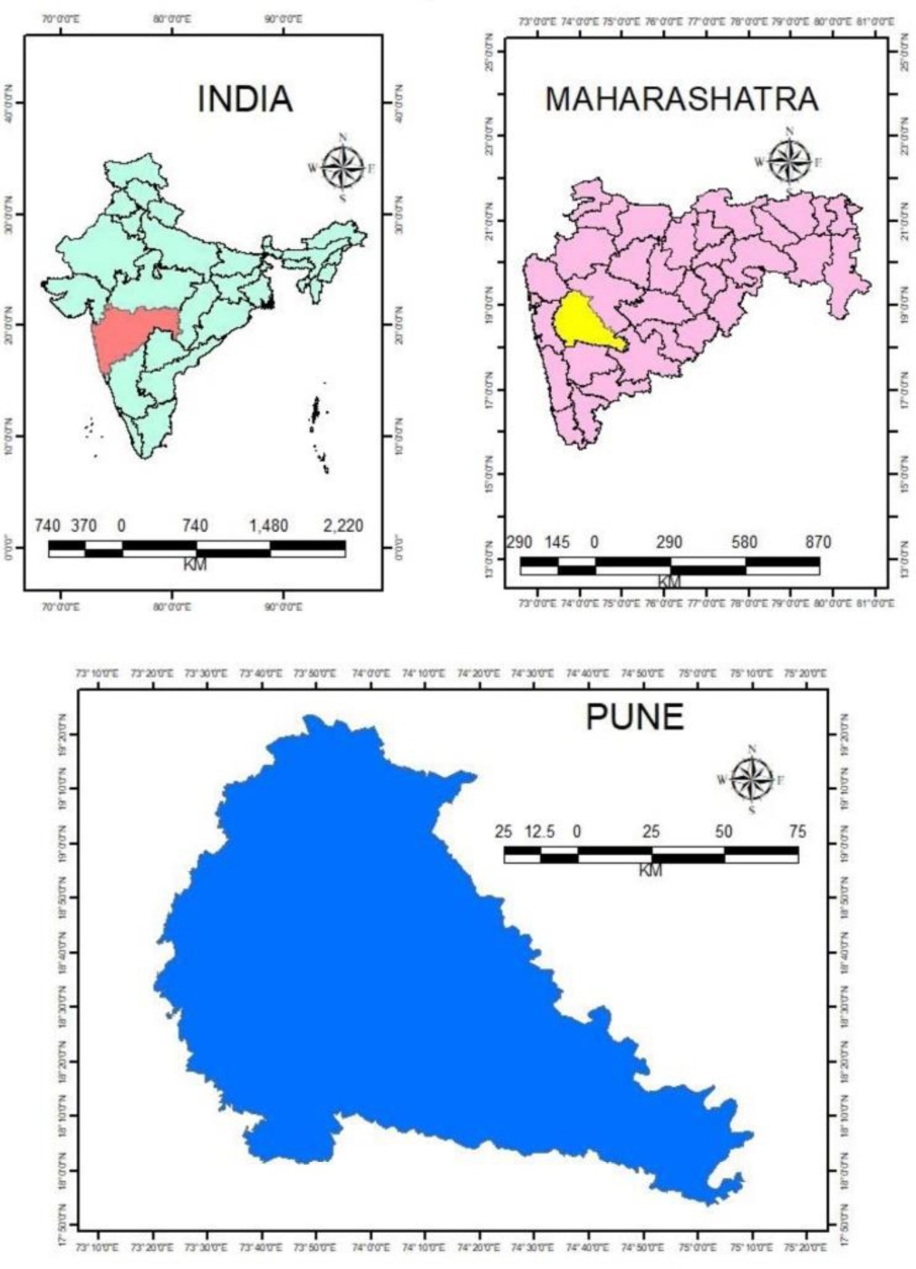
The study area is strategically important, and the upper Bhima River basin catchment (45,678 km²) is one of the important tributaries of the Krishna River in the upstream part of the basin in western Maharashtra state in India. The catchment is located between 16.5°-19.5° latitude and 73.0°-76.5° longitude. The elevation ranges from 414 m in the east to 1,458 m in the western Ghat mountains; 95% of the catchment is below 800 m and relatively flat. The location of Bhima basin in Pune is shown in Figure 2.

Fig. 2.

Location of study area.

The Hydrologic Engineering Center’s River Analysis System (HEC-RAS, V. 5.0.7) developed by the USACE is generally used for the study of flood analysis of numerous return periods. 1-D HEC-RAS hydrodynamic modeling is an applicable tool for deriving 1-D river hydraulic parameters including total discharge, water surface elevations (WSE), energy gradient elevation (EG), energy gradient slope, velocity, flow area, and Froude number at different channel sections, which help for better analysis. The applications are specifically planned for flood plain management and flood-insurance studies to estimate flood-way interruption and to reproduce estimated flood inundation in the study area. HEC-RAS demands a number of input variables for hydraulic analysis of the stream channel geometry and water flow. These parameters are used to create a series of cross-sections along the stream. In each cross-section, the locations of the stream banks are identified and used to divide the cross-section into segments of left flood-way, main channel, and right floodway. At every cross-section various input parameters are used to define elevation, shape, and relative position at a river station number, including lateral and elevation coordinates for all terrain points, left and right bank locations, downstream reach lengths between the left floodplain, stream center-line, and right floodplain of every adjacent cross-section, and Manning’s roughness coefficients for left, main channel, and right floodplains. Further, geometric descriptions of any hydraulic structures, such as bridges, culverts, and weirs for current study in flood modeling data for flood events of 2005 and 2017 were considered. A Bhima River stretch 67 of km with 595 cross-sections, each approximately 800 m long, was modeled. The primary data required for this modeling was collected from the Water Resource Department (WRD), Pune, Government of Maharashtra, National Hydrology Project (NHP)¹, Nasik Maharashtra, and Central Water Commission (CWC) water books. Manning’s roughness coefficients were selected according to Central Water Commission (CWC) guidelines; bank stations were marked with the help of RAS-Mapper and ArcGIS world imagery. Reach length data was also collected from WRD² at Pune in Maharashtra. River geometry was created as shown in Figure 3.

Fig. 3.

Geometry of Bhima River.

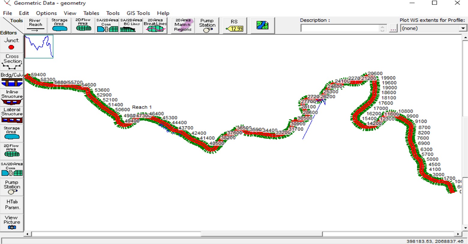
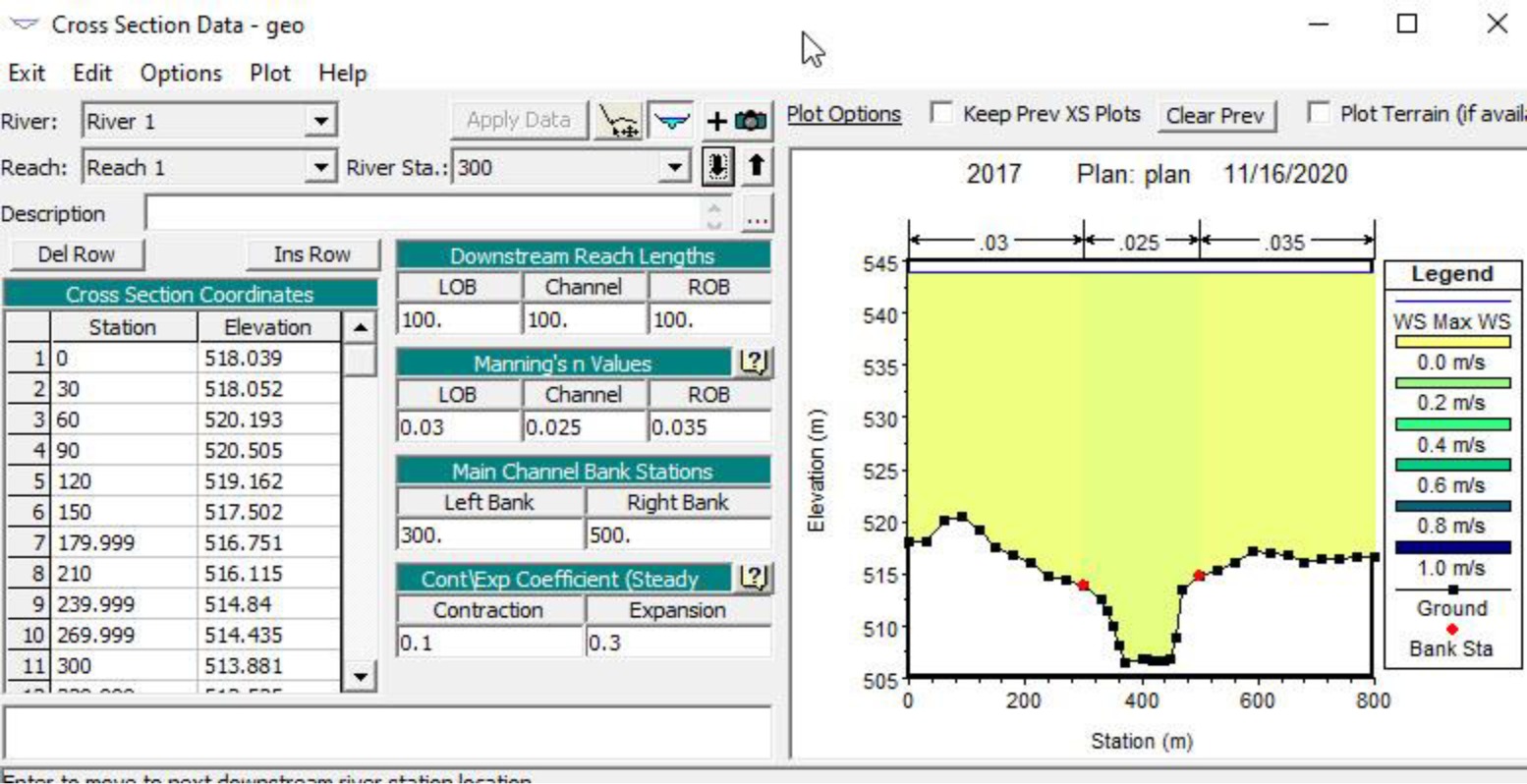
Manning’s coefficient reach lengths and bank stations were also used for each cross-section as shown in Figure 4. For hydrodynamic flow analysis, stage hydrographs for the period of July and August 2005 were used as downstream boundary conditions, and the flow hydrograph for the same period was used as the upstream boundary condition.

Fig. 4.

Cross-section details of the Bhima River channel.

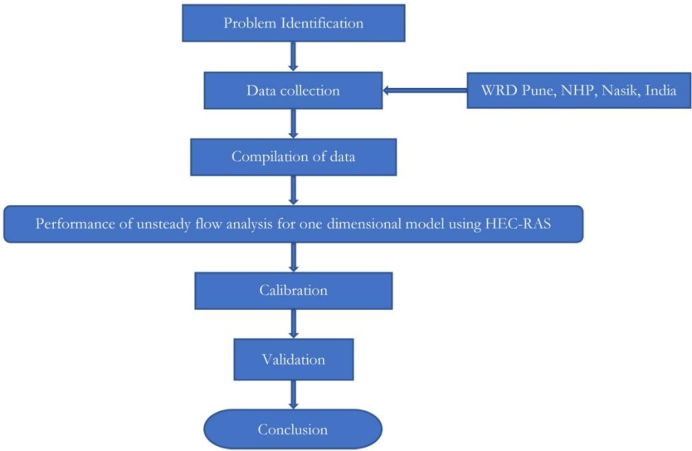
The flow data, and flow category with regime conditions are used to build up the model for the desired outcomes. The methodology followed is expressed in a flow chart (Figure 5).

Fig. 5.

Flowchart of methodology.

5. Data availability

Table 1 below gives the details of data types and sources of data used in this research paper on hydrodynamic flow modeling and the effect of roughness on river stage forecasting.

6. Hydrodynamic model calibration

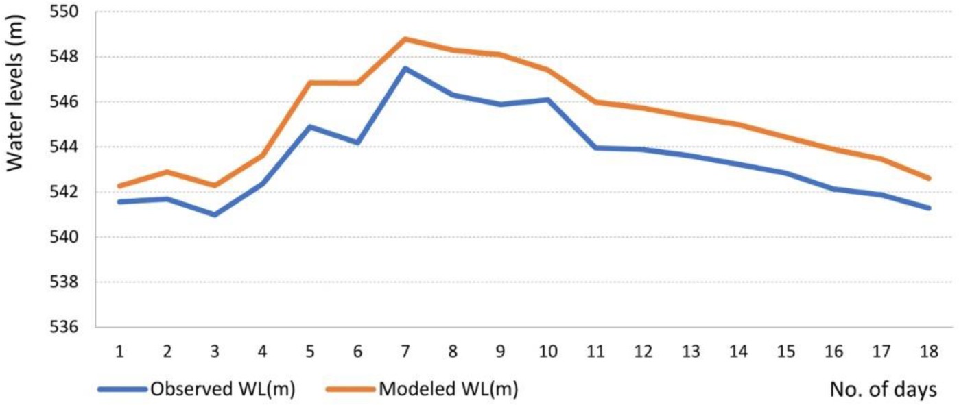
Calibration is the adjustment of a model's parameters so that it reproduces observed data to an acceptable accuracy. Roughness coefficients, i. e. Manning’s roughness coefficient (n) in this case, are among the main variables used in calibrating a hydraulic model. It is known that for a free-flowing river, roughness decreases with increased stage, and flow. However, if the banks of a river are rougher than the channel bottom, then the composite value of the roughness coefficient (n) will increase with increased stage. Deposits and debris can also play an important role in the roughness. When Manning’s n is increased in a particular area, then stage will increase locally, the peak discharge will decrease (attenuate) as the flood wave moves downstream, and the travel time will increase. The hydrodynamic model is calibrated using the flow hydrograph for the period of 20 July 2005 to 8 August 2005 as the upstream boundary condition and the stage hydrograph from 20 July 2005 to 8 August 2005 as the downstream boundary condition. Flow data from 2005 has been used for calibration of Manning's roughness coefficient ‘n’ at a time step of 24 hours. The flow and stage have been simulated using the daily hydrograph for two months from 20 July to 8 August 2005. Calibrations have been done using Manning's roughness coefficient for values ranging from 0.015 to 0.040. Subsequently, final control parameters obtained from calibration have been used for validation in the Bhima River basin. Manning's roughness coefficient (n)was fixed as 0.025 for the main channel, 0.03 for the left floodplain, and 0.035 for the right floodplain. The comparison of observed and simulated stage hydrograph at Phulgaon gauging station (Latitude: 18°40'01", Longitude: 74°00'08)³, using the specified values of n, are shown in Figure 6.

Fig. 6.

Calibrated water level profiles (stages) at Phulgaon gauging station (from 20 July 2005 to 8 August 2005).

7. Hydrodynamic flow validation

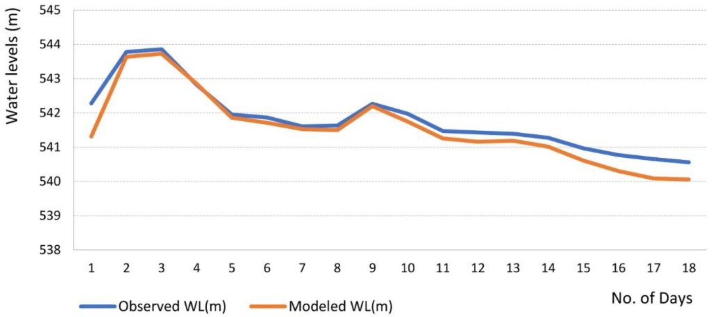
Model validation involves testing of a model with observed field data. This data set is an independent source for channel flow, distinct from the data used to calibrate the model. The calibrated hydraulic model has been used to validate the flow for the year 2017⁴. The comparison of observed and simulated flow hydrographs at Phulgaon gauging station in the basin is shown in Figure 7.

Fig. 7.

Validation water level profiles (stages) at Phulgaon gauging station (from 20 July 2005 to 8 August 2005).

8. Model performance evaluation

Performance of the hydraulic simulation model has been evaluated using the statistical performance indicators coefficient of determination (R²) (Equation 11) and root mean square error (RMSE) (Equation 12). The R² statistic describes the degree of agreement between simulated and measured water levels in the analysis. R² ranges from 0 to 1, with higher values indicating less error variance; typically values greater than 0.5 are considered acceptable in flow modeling (Legates, McCabe 1999; Moriasi et al. 2007).

where yi actual/observed data at i^th value; ŷi simulated result at ith value; n – total number of data; ȳ – mean value of n data.

The root-mean-square deviation (RMSD) or root-mean-square error (RMSE) is a commonly used to express the quantity of the differences between values predicted by a model and the values observed.

where: i^th variable, N – number of data points; X_i – observed values; Xi−– simulated values.

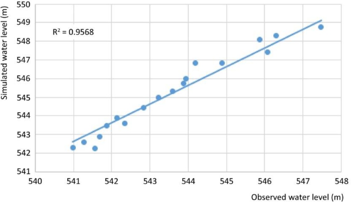
In calibration of the model, the coefficient of determination R² and lowest root mean square error (RMSE) were 0.9568 (Fig. 8) and 0.3099, respectively, which indicate that the simulated river stages are close to the observed stages.

Fig. 8.

Simulated river stages versus observed river stages.

9. Concluding remarks

This paper discusses 1-D hydrodynamic modeling developed using the Hydrologic Engineering Center’s River Analysis System (HEC-RAS) and a geographical information system. The model is calibrated for the Phulgaon gauging station using the flow hydrograph during 20 July 2005 to 8 August 2005. Calibrations and validations for various values of Manning’s roughness coefficient (n) were done, and observed and simulated water levels were compared. Values of n = 0.025 for the main channel, 0.03 for the left flood-plain and 0.035 for the right floodplain gave optimum results for simulated water levels. The hydrodynamic flow model validation has the highest R² and lowest RMSE. These statistics indicated that the simulated values of water levels are in close agreement with the observed value of water levels. hydrodynamic flow modelling of the Bhima River basin in India using HEC-RAS demonstrates satisfactory validity for the selected values of n.