2.1. Study area

The Prypiat River is a large right-hand tributary of the Dnipro River, which flows through parts of Belarus and Ukraine. It originates in the west of Ukrainian Polissia, thence 204 km downstream it crosses the border into the Republic of Belarus, where it flows for more than 500 km along the Polissia lowland. The last 50 km of the Prypiat River flows again into the territory of Ukraine and into the Kyiv reservoir (Dnipro River) (Fig. 1) (Kalinin, Obodovskyi 2003).

Fig. 1.

The location of the Prypiat River basin within Ukraine and the 29 water gauges and 17 meteorological stations within its catchment (the numbering of stations is based on Tables 1 and 2).

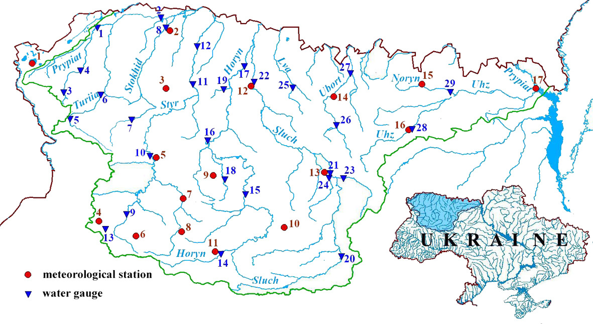
The total length of the river is 761 km, and the catchment area is 121,000 km². Within the borders of Ukraine, the length of the river is 254 km, the catchment area is 68,370 km², and it is the greater right-bank part of the Prypiat River basin (Kalinin, Obodovskyi 2003; Vishnevsky 2000). The Ukrainian part of the Prypiat River basin borders the Western Bug River to the south and west, the Dniester and Southern Bug Rivers to the south, and the Dnipro River to the east and southeast. The Prypiat River has 14 right-bank tributaries, of which the Horyn, Styr, and Uzh rivers are the largest. The right-bank river basin is located in Polissia, which is characterized by lowland relief, wide waterlogged river valleys, a positive moisture balance, and a wide distribution of sod-podzolic and swampy soils. The relief of Polissia is a large plain with altitudes that rarely exceed 150-200 m (Vasylenko 2015).

According to the classification by Köppen (1936), the climate of the Pripyat basin is temperate-continental with warm and humid summers and fairly mild winters. The territory of the basin is mainly under the influence of Atlantic air masses, as well as Arctic air, which brings cooling throughout the year. Warming in winter and hot weather in summer are caused by southern tropical air masses that, although rarely, sometimes reach Polissia. Summer, especially in the second half, is characterized by cool and often rainy weather. Autumn is often rainy, and spring is more prone to unstable weather, which is explained by the change of various air masses, cyclones, and anticyclones.

The warmest month in the basin is July, and the coldest is January. Sometimes there are shifts in heat and cold peaks, respectively, in August and February. The mean temperature in July is 18-19°C, and in January is from –4.5°C to –7°C (Kalinin, Obodovskyi 2003; Strutynska, Grebin 2010).

Cyclones coming from the Atlantic bring with them a significant amount of precipitation, the average annual amount of which fluctuates within significant limits and is 600-700 mm on the right bank. The largest amount of precipitation falls in July-August: in dry years, as little as 350 mm, and in wet years up to 1000 mm or more (Kalinin, Obodovskyi 2003).

Ice phenomena of the Prypiat River in the form of shore ice and grease usually appear in late October-November. Autumn ice drift on the river, on average, begins in the last 10 days of November or early December, but in some years, it is observed near the end of October and is sometimes delayed until mid- or late-December (Strutynska, Grebin 2010).

2.2. Data

Trend analysis of air temperature was based on data from 17 meteorological stations (Fig. 1). Mean monthly air temperatures for November, December, and March were calculated from the earliest observations to 2020, inclusive (Table 1). These data were compiled from the Meteorological Yearbooks published by the Borys Sreznevsky Central Geophysical Observatory (Kyiv, Ukraine). November, December, and March were chosen because, in most cases, in the rivers of the basin ice formation and freeze-up occur in November and December and ice break-up and melting occur in March (Afteniuk 2020). The mean duration of the records is 80 years. The longest record covers 96 years (Novohrad-Volynskyi stations); the shortest covers 71 years (Olevsk stations).

Ice data from 29 water gauges in the Prypiat River basin were compiled from the Hydrological Yearbooks, also published by the Borys Sreznevsky Central Geophysical Observatory (Fig. 1, Table 2). Data were used from the earliest observations to 2020, inclusive. The mean duration of the records is 78 years. A large majority of records cover more than 70 years. Most observations begin in the 1920s-1930s, with the latest beginning in 1985. Thus, the longest record has observations for 96 years (Sluch River, Novohrad-Volynskyi city), and the shortest record has observations for 35 years (Ustia River, Kornyn village).

Note that the longest records of air temperature and ice phenomena have gaps of several years. These gaps are small compared to the total duration of the records and allow us to carry out trend analysis. In addition, the results of such an analysis can be used to determine the probabilistic characteristics of ice phenomena for which information on all observed phenomena is important.

For each water gauge and each winter period (October to April), six data classes were extracted:

The date after which the ice lasted for 3 or more days was taken as the appearance date of ice. In cases when icing was interrupted, i.e., the water surface was clear of ice, and the duration of such an interruption was from 1 to 3 days, the period was considered continuous. The ice break-up date was determined by the dates of the beginning of melting. The date of disappearance was defined as the last date when ice was observed. This approach objectively reflects the real situation of ice phenomena on rivers.

2.3. Methodology

Statistical and graphical methods were used to assess trends in air temperature and ice dynamics in the Prypiat River basin in Ukraine. Given the features of the hydrological and meteorological series of observations (non-normal distributions, seasonally and serially correlated), the Pearson method and nonpara-metric Mann-Kendall test were used (Kundzewicz, Robson 2004; WMO 2009). The trend equation in the time series and the correlation coefficient between variables were determined by the Pearson method. Estimation of statistical significance in trends employed the nonparametric Mann-Kendall test (Mann 1945; Kendall 1975). The calculations were carried out using RStudio Software (version 1.4.1717) (R Core Team 2017). If the statistical characteristics (mean and variance) of time-series do not change over time, then the time series exhibits stationarity (i.e., there is no time trend) (Robson 2002).

Graphical analysis has been widely recommended for confirming the results of trend analysis by statistical tests (Kundzewicz, Robson 2000, 2004; WMO 2009; Gorbachova 2016; Şen 2017; Hussain 2019; Onyutha 2021). This approach is especially important when statistical tests do not have unambiguous interpretations, e.g., when only one statistical test is used, or when several statistical tests with the same properties are used (Robson 2002; WMO 2009; Gorbachova, Bauzha 2013).

Graphic methods such as mass curve analysis, double mass analysis, and residual mass curve are the most widely used in these investigations (Gorbachova 2016). Klemeš (1987) and Gorbachova (2016) reported that at the end of the 19th and during the 20th centuries these methods were developed by Rippl (1883), Schoklitch (1923), Novotný (1925), Merriam (1937), Kohler (1949), Weiss and Wilson (1953), Searcy and Hardison (1960); Ehlert (1972). The present investigation employed the mass curve, residual mass curve, and combined graphs. This methodological approach was developed by Gorbachova (2014, 2016) and applied to evaluate river flow trends (Bauzha, Gorbachova 2017; Gorbachova et al. 2018; Zabolotnia et al. 2019; Romanova et al. 2019; Melnyk, Loboda 2020; Zabolotnia et al. 2022), also including ice dynamics. (Gorbachova, Khrystyuk 2012; Gorbachova 2013; Rachmatullina, Grebin 2014).

The mass curve is used to detect changes in hydrometeorological characteristics under the influence of anthropogenic factors and climate change, which can appear on the curve in the form of “jumping,” “emissions,” or unidirectional deviation. Residual mass curves and combined graphs were used for the assessment of spatiotemporal fluctuations of hydrometeorological characteristics. The residual mass curve supports analysis of trends in hydrometeorological characteristics over time: periods of change, cyclical fluctuations, and their characteristics (phases of increase and decrease, their duration, synchronicity, in-phase). In turn, the synchrony or asynchrony of long-term fluctuations of hydrometeorological characteristics in the different observation series can be defined by combined graphs. Moreover, the residual mass curve analysis of hydrometeorological characteristics supports determining the stationarity of data series, i.e., the sustainability of the mean value of the time series over time. The mean value of the time series is stable in the presence of at least one full closed cycle (increase and decrease phases) of long-time fluctuations. The methodological recommendations for the use of graphic methods are described in detail by Gorbachova et al. (2018).

For graphical analysis of ice dynamics, dates for initial values for their numeric presentation were taken to be the earliest dates of the appearance (or disappearance) of river ice.

3.1. Air temperature

Analysis of data from the observation series of mean monthly air temperature for November, December, and March for stationarity with the Mann-Kendall test showed statistically significant trends (p ≤ 0.05) for all observations in March (Table 3). In November, 8 observation series of the mean monthly air temperature were stationary, and in December, only 4 series were stationary. For a clearer understanding and confirmation of the results according to the Mann-Kendall statistical test, the study evaluated the homogeneity, stationarity, and fluctuations of the observation series using graphic methods.

The mass curves of the mean monthly air temperature show that all observation series are homogeneous because the curves do not display “jumping,” “emissions,” or unidirectional deviation (Fig. 2, upper row).

Fig. 2.

Mass curves (upper row) and residual mass curves (bottom row) of mean monthly air temperature for November (on the left side), December (in the center), and March (on the right side) for some meteorological stations (1 – Manevichi, 2 – Dubno, 3 – Shepetivka, 4 – Korosten) in the Prypiat River basin (within Ukraine); K = temperature in degrees Kelvin.

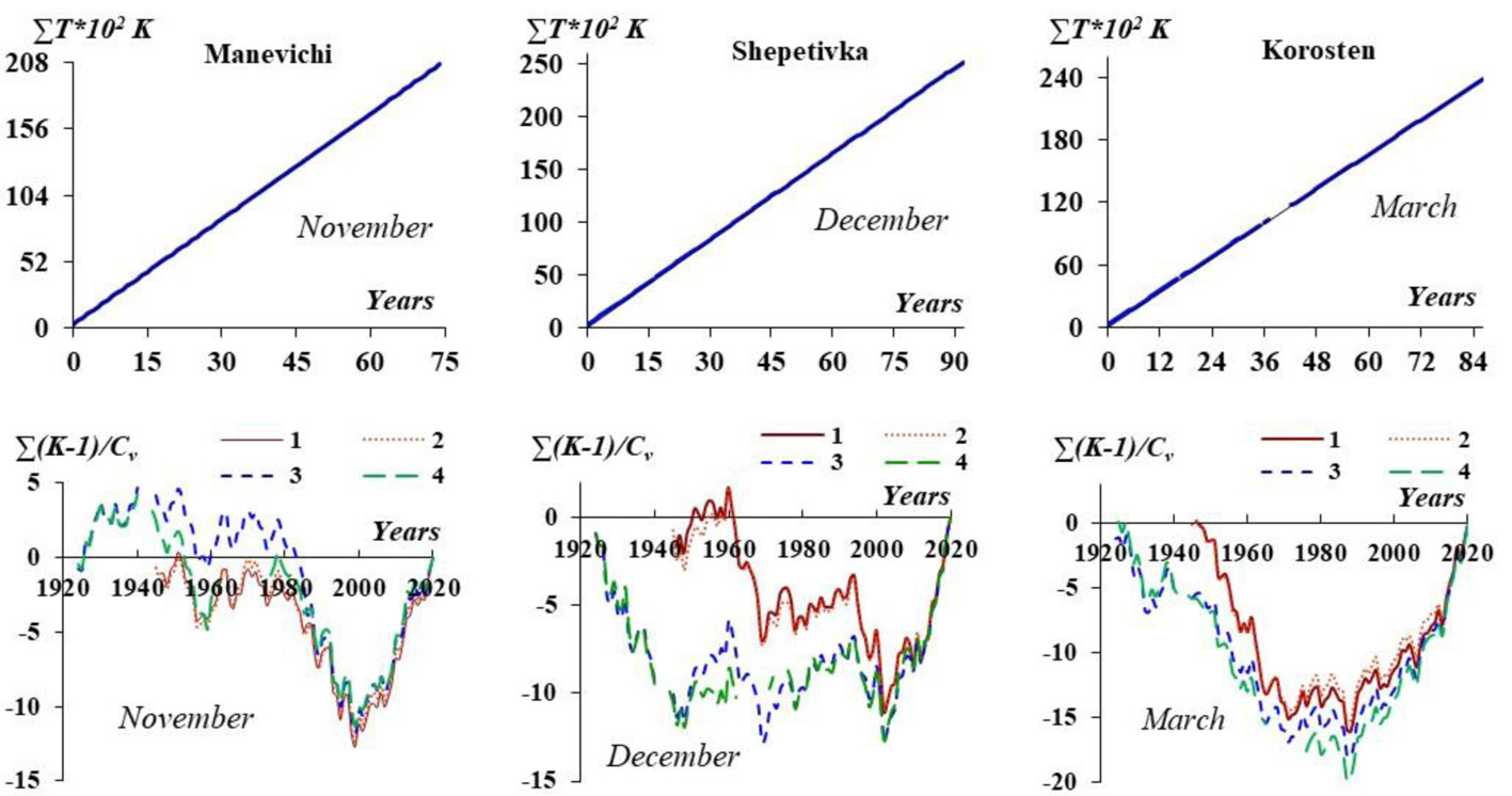
The forms of the residual mass curves indicate that the observation series of the mean monthly air temperature are characterized by cyclical fluctuations of different durations (Fig. 2 bottom row). In November, the series of mean monthly air temperatures have several short complete cycles of fluctuations that lasted from the beginning of observations, i.e., from the beginning of the 1920s until 1978. Their mean duration was 9 years. The long-term cycle of fluctuations began after 1978, namely, the cooling phase was from 1978 to 1999, and the warming phase began after 1999, continuing to the present, and the end of which cannot be predicted.

In December, the cooling phase was from the beginning of the 1920s until 1948. After 1948, two relatively short but well-defined cycles of fluctuations were observed. Their durations were 21 years (1948-1969) and 33 years (1970-2002). The warming phase began after 2002. In March, the mean monthly air temperature series have a clearly defined cooling phase and a warming phase of long-term cyclical fluctuations. The cooling phase started from the beginning of observations and lasted until 1988. The warming phase began after 1988. Cycles of short fluctuations are traced both for the cooling phase and for the warming phase. However, such short fluctuations have a rather short duration, i.e., 4-6 years on average and a small amplitude.

The beginning of the cooling phase in the air temperature observation series can be determined clearly only in November. For all other series, the cooling and warming phases are incomplete because the beginning of the observations took place when the cooling phase was already ongoing, and the warming phase is still ongoing. So, for defining constant average values, all observation series are not representative. Nonetheless, the observation series of mean monthly air temperature still have phases of cooling and warming long-term cyclical fluctuations, although they are incomplete. Such a series can be classified as quasi-stationary.

Long-term cyclic fluctuations of the mean monthly air temperature in November, December, and March are characterized by synchronicity and in-phase, indicating homogeneity of air temperature dynamics throughout the Pripyat River basin.

3.2. Ice dynamics

The analysis of ice occurrence and freeze-up observations for stationarity according to the Mann-Kendall test showed that most of the series are non-stationary (Table 4). At the same time, the observation series of ice-appearance date and freeze-up did not have the same trends. Twelve observation series for ice-appearance date and 17 observation series for the date of freeze-up turned out to be stationary.

Mass curves of the ice-appearance date and freeze-up on rivers and their duration show that the cumulative values initially deviate from a straight line, but then change direction and cross the straight line and seem to form a kind of arc (Figs. 3 and 4, upper rows).

Fig. 3.

Some mass curves (upper row) and residual mass curves (bottom row) of the ice-appearance date (on the left side), ice -disappearance date (in the center), and ice duration (on the right side) in the Prypiat River basin within Ukraine: 1 – Prypiat River – Liubiaz village, 2 – Styr River – Mlynok village, 3 – Sluch River – Hromada village, 4 – Uzh River – Korosten city; σD = standard deviation of the observation series of the ice appearance and disappearance dates.

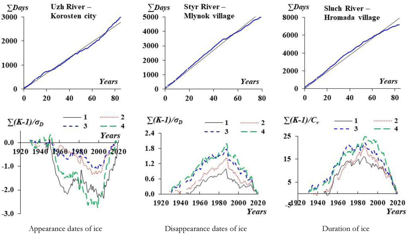
Fig. 4.

Mass curves (upper row) and residual mass curves (bottom row) of the dates of freeze-up (on the left side), break-up dates of freeze-up (in the center), and duration of freeze-up (on the right side) in the Prypiat River basin within Ukraine: 1 – Prypiat River – Liubiaz village, 2 – Styr River – Mlynok village, 3 – Sluch River – Hromada village, 4 – Uzh River – Korosten city; σD = the standard deviation for the observation series of the freeze-up appearance and break-up dates.

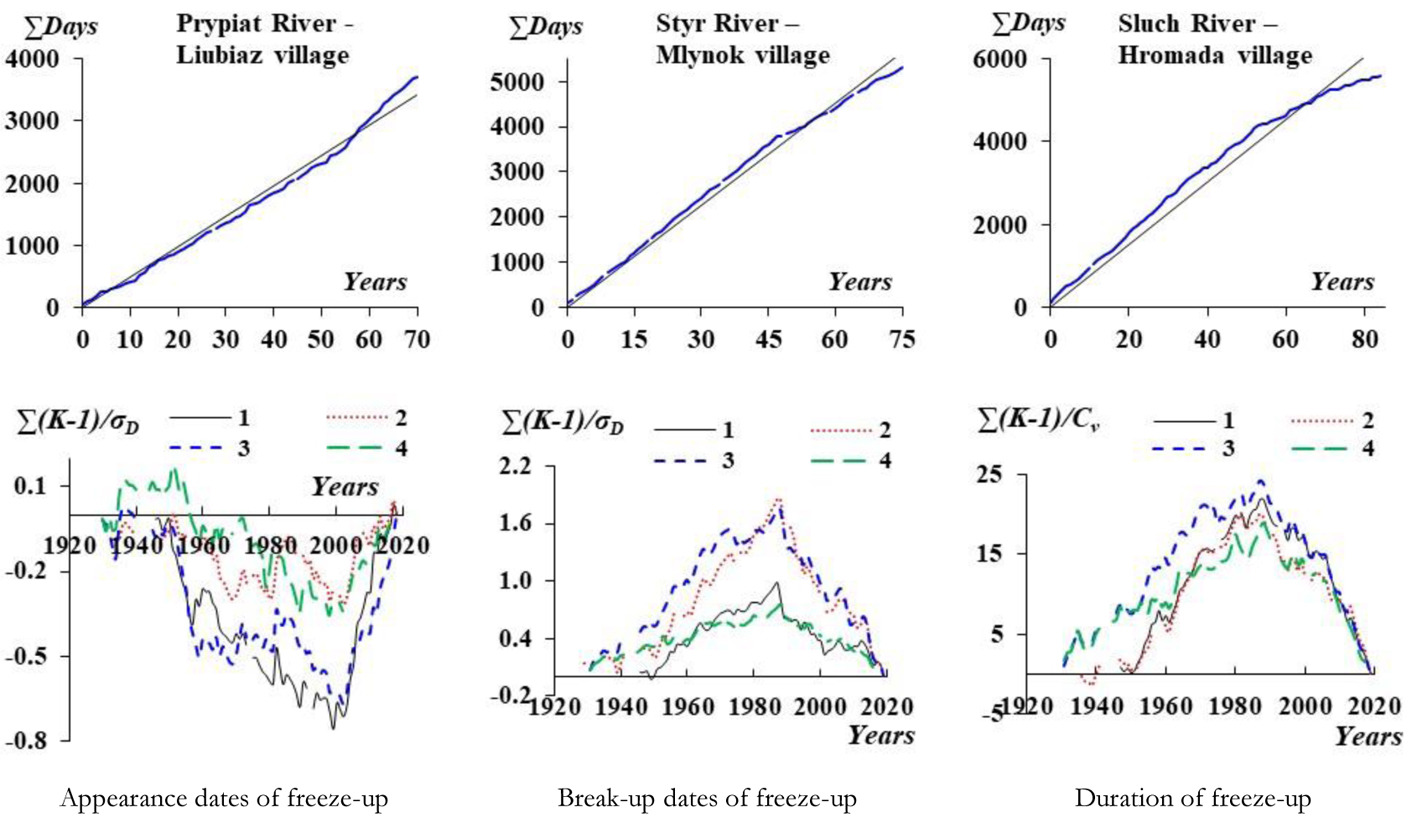
This type of mass curve indicates the absence of a unidirectional stable tendency in the series of ice dynamics. So, the form of the mass curves shows that the observation series have inflection points, after which the trends change.

The analysis of residual mass curves showed that the observation series for which the ice-appearance date and the freeze-up date occurred in November show a transition from a decreasing phase to an increasing phase in long-term cyclical fluctuations in 1999 (Figs. 3 and 4, bottom row). If the formation of ice and freeze-up on the rivers occurred in December, then such a transition was in 2002. A different trend is characteristic for the break-up date of freeze-up and the ice-disappearance date, i.e., the observations began in the increasing phase, changing into the decreasing phase after 1988. The observation series of the duration of freeze-up and ice occurrence have similar tendencies. Therefore, the presence in the observation series of the phases of increasing and decreasing long-term cyclical fluctuations determines the arc-shaped form of the mass curves of ice phenomena and their duration. It is clear that such observation series are quasi-homogeneous and quasi-stationary.

The analysis of cyclic fluctuations of the mean monthly air temperature in November, December, and March, along with cyclic fluctuations of ice-appearance main phases and their duration shows that air temperature is the main factor affecting ice formation in rivers and determines their long-term tendencies. Thus, the warming phase that began in 1999 for November and 2002 for December, determined the increasing phase of the ice-occurrence dates and freeze-up dates on rivers, i.e., icing and freeze-up are forming on the rivers later in the year. The warming phase for March began after 1988. This causes earlier ice break-up and disappearance on the rivers (decreasing phase). As a result of these dynamics, the duration of ice occurrence and freeze-up on the rivers in the Pripyat River basin has decreased.