1. Background and motivation
Precipitation is a fundamental component of the hydrological cycle, supporting agricultural productivity, water resource management, and ecosystem sustainability. Sudan exhibits pronounced climatic variability, ranging from hyper-arid desert conditions in the north to semi-humid savannahs in the south. Understanding precipitation patterns and variability is therefore essential for mitigating drought impacts, ensuring food security, and developing effective climate adaptation strategies in this highly climate-sensitive region. However, the sparse and uneven distribution of ground-based meteorological stations across Sudan limits the accurate reconstruction of historical precipitation records and constrains the assessment of climate-related risks (Funk et al. 2015).
Global Climate Models (GCMs), including those developed under the Coupled Model Intercomparison Project Phase 6 (CMIP6), provide valuable insights into past and future climate conditions. Nonetheless, these models often exhibit systematic biases when simulating regional precipitation, particularly in arid and semi-arid regions (Eyring et al. 2016). Such biases can significantly affect the reliability of model-based precipitation estimates and increase uncertainties in hydrological modeling and climate impact assessments. To overcome these limitations, bias correction techniques are widely applied to statistically adjust GCM outputs, aligning them more closely with observed data (Gudmundsson et al. 2012; Maraun 2013).
Despite the growing use of bias correction methods, comprehensive evaluations focusing specifically on Sudan remain scarce (Gebrechorkos et al. 2019). The country’s steep climatic gradients and high spatial and temporal rainfall variability pose unique challenges for model calibration and correction. While studies across East Africa have shown that bias adjustment improves model performance, systematic assessments for Sudan, where observational networks are particularly limited, are still lacking. This gap highlights the need for detailed regional analyses to identify the most effective bias correction techniques for improving precipitation simulations and supporting climate resilience planning (Siddig et al. 2022).
2. Objectives and scope
Bias correction techniques enhance the reliability of climate model outputs by reducing systematic errors and improving alignment with observed climatology. Such adjustments are especially important for General Circulation Model (GCM) analyses, where uncorrected biases can substantially limit the usefulness of model projections. This study evaluates the performance of four widely used bias correction methods: Empirical Quantile Mapping (EQM), Gamma Quantile Mapping (Gamma-QM), Local Intensity Scaling (LOCI), and the Delta Method. These methods were applied to monthly precipitation simulations from ten CMIP6 models over Sudan during the 1991-2014 historical period. The Climate Hazards Group InfraRed Precipitation with Station data (CHIRPS) is the observational benchmark for assessing each method’s effectiveness. Model performance is quantified using multiple complementary statistical metrics, including the Pearson correlation coefficient, centered root-mean-square deviation (CRMSD), mean bias, and Kling–Gupta Efficiency (KGE). In addition to evaluating bias correction methods, the study identifies the best-performing CMIP6 models for annual and seasonal (March-May and June-September) periods, providing guidance on the most reliable simulations for capturing spatial and temporal precipitation variability across Sudan. This study is novel in its regional focus on Sudan and in systematically comparing quantile-based and scaling-based bias correction techniques. By integrating statistical performance metrics with spatial diagnostics, it enables a comprehensive evaluation of model performance, thus providing practical guidance for applying bias correction and selecting appropriate climate models for hydroclimatic studies across East Africa.
3. Study area and data
3.1. Study area
This study focuses on Sudan, the third-largest country in Africa, located between approximately 8°–23.5°N and 21°E–39°E. The country exhibits a pronounced climatic gradient, transitioning from hyper-arid desert conditions in the north to semi-arid and savanna environments in the south (Fig. 1), with elevation decreasing from the highlands in the east and south to the northern plains. Correspondingly, precipitation patterns are highly variable across the country, with northern regions receiving little rainfall and southern regions experiencing substantially higher totals, as shown by CHIRPS observations.
Fig. 1.
Maps of Sudan with geographical coordinates. Panel (a) shows the shaded-relief elevation derived from the digital elevation model (DEM), and panel (b) shows the mean annual precipitation (mm/year) from CHIRPS, averaged over 1991-2014 at 0.25° spatial resolution.
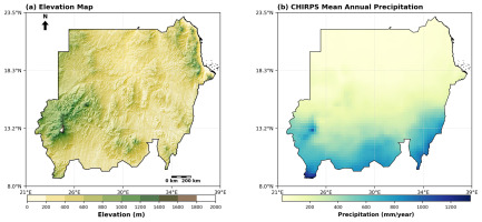
Rainfall in Sudan is strongly seasonal, primarily driven by the north-south migration of the Intertropical Convergence Zone (ITCZ), with most precipitation occurring between June and September (Nicholson 2018; RCCC 2022). This spatial and temporal variability has important implications for agriculture, water resources, and disaster risk management. Northern Sudan frequently faces prolonged droughts, while southern areas are more susceptible to intense rainfall events that can trigger seasonal flooding (RCCC 2022).
Sudan’s sensitivity to climate variability and change, combined with environmental and socio-economic pressures, makes it a valuable case study for evaluating climate models and assessing the effectiveness of bias correction techniques in reproducing historical precipitation patterns (Jackson et al. 2020).
3.2. Data
This study employs both observational and climate model datasets to evaluate bias correction techniques for monthly precipitation over Sudan. Observational data are sourced from the CHIRPS dataset, a high-resolution gridded product that integrates satellite-derived precipitation estimates with in-situ rain gauge measurements (Funk et al. 2015). CHIRPS provides near-global coverage at 0.05° spatial resolution, making it particularly valuable in regions with sparse or unevenly distributed observational networks, such as Sudan (Nicholson 2018; ICPAC 2020). Its reliability has been demonstrated in multiple studies across East Africa, including evaluations of historical precipitation variability, seasonal rainfall patterns, and extreme events, establishing CHIRPS as a robust benchmark for climate model evaluation in the region (ICPAC 2020).
For this analysis, monthly CHIRPS precipitation data from January 1991 to December 2014 were aggregated to a 0.25° resolution to match the climate model outputs. Precipitation values are expressed in mm month -¹, and the data were spatially clipped to Sudan’s national boundaries using a country-level shapefile. The combination of high spatial resolution, integration of ground-based observations, and demonstrated reliability makes CHIRPS a suitable reference for assessing CMIP6 precipitation simulations and the effectiveness of bias correction techniques over Sudan. Although CHIRPS is available through 2020, the evaluation was restricted to 1991-2014 to align with the CMIP6 historical simulations.
Table 1.
CMIP6 models used in this study, with their institutions, countries, approximate horizontal resolution, sensitivities and key reference.
| No. | Model ID | Institute/Country | Resolution (°) | Sensitivity | Reference |
|---|---|---|---|---|---|
| 1 | AWI-CM-1-1-MR | Alfred Wegener Insti-tute / Germany | ~1.0° | Strong ocean–sea-ice coupling,af-fecting moisture transport and tropi-cal rainfall. | Semmler et al. (2019) |
| 2 | EC-Earth3 | EC-Earth Consortium / Europe | ~1.0° | Updated convection and aerosol–cloud schemes,improving monsoon rainfall representation. | Döscher et al. (2022) |
| 3 | GFDL-ESM4 | NOAA Geophysical Fluid Dynamics Labor-atory / USA | ~1.0° | Improved cloud microphysics, radia-tion, and land–atmosphere coupling shaping East African rainfall. | Heldet al. (2019) |
| 4 | HadGEM3-GC31-LL | Met Office Hadley Centre / UK | ~1.25° | Complex convection and cloud schemes; high sensitivity in ITCZ/tropical rainfall. | Williams et al. (2018) |
| 5 | INM-CM4-8 | Institute for Numerical Mathematics / Russia | ~2.0° | Simplified cloud and convection pro-cesses leading to weaker precipitation feedback. | Volodin et al. (2018) |
| 6 | KACE-1-0-G | Korea Meteorological Administration / South Korea | ~1.25° | Updated KIM convection scheme enhancing tropical rainfall timing and intensity. | Byun et al. (2019) |
| 7 | MIROC6 | AORI / NIES / JAM-STEC / Japan | ~1.4° | Enhanced entrainment–detrainment convection,improving monsoon pre-cipitation. | Tatebe et al. (2019) |
| 8 | MRI-ESM2-0 | Meteorological Re-search Institute / Japan | ~1.1° | Advanced cloud microphysics and precipitation formation,improving rainfall distribution. | Yukimoto et al. (2019) |
| 9 | NESM3 | Nanjing Univ. of Infor-mation Science / China | ~1.0° | Strong cloud feedback and updated boundary-layer scheme affecting monsoon variability. | Cao et al. (2018) |
| 10 | TaiESM1 | Research Center for Environmental Changes / Taiwan | ~1.0° | Enhanced aerosol–cloud–convection interactions influencing spatial rain-fall patterns. | Lee et al. (2020) |
Climate data were obtained from ten carefully selected CMIP6 global climate models, chosen based on spatial resolution, data availability, and relevance to East Africa (Eyring et al. 2016). Model outputs were converted to mm month-¹, regridded to 0.25° spatial resolution, and clipped to Sudan’s national boundary to ensure consistency with CHIRPS observations (Gudmundsson et al. 2012). These ten models correspond to a subset of 23 CMIP6 models previously evaluated over the IGAD region, including Sudan, and identified in the literature as demonstrating relatively high skill in reproducing precipitation totals, seasonal cycles, and extreme events (Ayugi et al. 2022). Their documented performance makes them particularly suitable for climate impact assessments and hydrological studies in the region.
4. Methodology
4.1. Bias correction methods
To address systematic biases in CMIP6 precipitation outputs, four bias correction techniques were applied at a monthly time scale: Empirical Quantile Mapping (EQM), Gamma Quantile Mapping (Gamma-QM), Local Intensity Scaling (LOCI), and the Delta Method. These methods span both parametric and non-parametric approaches, capturing a broad methodological spectrum relevant to precipitation adjustment (Teutschbein, Seibert 2012).
Empirical Quantile Mapping (EQM)
EQM is a non-parametric bias correction approach that aligns the empirical cumulative distribution function (CDF) of the simulated precipitation with that of the observations (Maraun 2016). The corrected precipitation is computed as:
where Fmod,emp and
Gamma Quantile Mapping (Gamma-QM)
Gamma-QM is a parametric technique that assumes precipitation follows a gamma distribution.
The distribution parameters are estimated via maximum likelihood for both model and observations. The correction is expressed as:
where Fmod,Γ and
Local Intensity Scaling (LOCI)
LOCI preserves the occurrence of dry months while correcting precipitation intensity. For months where Praw < T (with T = 1 mm/month in this study), precipitation remains zero; otherwise, it is scaled by:
where the scaling factor is:
where μobs,>T and μmod,>T are the wet-month average precipitation values from observations and models, respectively (Schmidli et al. 2006). This approach preserves dry-month statistics, corrects systematic intensity biases, and is particularly suitable for arid and semi-arid regions such as Sudan.
Delta Method
A straightforward bias adjustment method applying a monthly multiplicative correction:
where
4.2. Performance evaluation metrics
To quantify the effectiveness of the bias correction techniques, a set of complementary statistical measures was employed to compare simulated precipitation against the CHIRPS observational reference. The Pearson correlation coefficient (r) evaluates the strength and direction of the linear association between modeled and observed values. The Root Mean Square Error (RMSE) captures the overall magnitude of deviations, reflecting the typical difference between simulations and observations. The Mean Bias (MB) indicates the systematic tendency of models to overestimate or underestimate precipitation relative to observations.
The Pearson correlation coefficient (r) quantifies the strength and direction of the linear relationship between simulated (xi) and observed (yi) precipitation:
where
The Root Mean Square Error (RMSE) provides a measure of the average magnitude of deviations between simulations and observations, reflecting the overall accuracy of the model:
The Mean Bias (MB) indicates systematic overestimation or underestimation by the model:
A key integrative metric, the Kling–Gupta Efficiency (KGE), synthesizes three critical aspects of a model: performance correlation, variability, and mean bias, into a single score. Using the revised formulation (Kling et al. 2012), the KGE is calculated as:
Here, r represents the Pearson correlation coefficient, which quantifies the linear association between simulated and observed precipitation. The term
4.3. Uncertainty quantification and robustness assessment
To assess the reliability of the performance metrics and the robustness of bias correction methods, a non-parametric bootstrapping approach was implemented with 1,000 resampled datasets to estimate 95% confidence intervals, providing a rigorous evaluation of statistical uncertainty for each metric (Efron, Tibshirani 1993). In addition, sensitivity analyses were conducted to examine both seasonal (March-May and June-September) and spatial variability in method performance across Sudan (Saltelli et al. 2008). Statistical significance testing was applied to determine whether observed improvements in bias-corrected outputs relative to raw simulations were meaningful, ensuring that conclusions drawn are robust and defensible (Wilks 2011).
5. Results
5.1. Model evaluation
The initial evaluation of raw CMIP6 precipitation simulations over Sudan was conducted through direct comparison with CHIRPS observational data for the period 1991-2014. Four complementary statistical metrics were computed to quantify model performance: Centered Root Mean Square Difference (CRMSD), mean bias, Pearson correlation coefficient (r), and Kling–Gupta Efficiency (Wilks 2011; Kling et al. 2012). CRMSD measures the magnitude of pattern errors after removing the mean bias, bias quantifies systematic overestimation or underestimation, the correlation coefficient assesses the temporal agreement between model and observations, and KGE integrates correlation, variability, and bias into a single skill metric.
Substantial variability was observed among the ten CMIP6 models when expressed relative to the CHIRPS mean precipitation. Correlation coefficients ranged from 0.72 to 0.95, with EC-Earth3 (r = 0.95), NESM3 (r = 0.93), INM-CM4-8 (r = 0.92), KACE-1-0-G (r = 0.92), and MIROC6 (r = 0.92) exhibiting the strongest temporal agreement. Relative CRMSD values, expressed as a percentage of the CHIRPS mean, ranged between 10.87% (EC-Earth3) and 25.31% (MRI-ESM2-0), highlighting marked differences in the models’ ability to reproduce observed temporal variability. Mean bias analysis revealed that most models tended to underestimate rainfall, particularly AWI-CM-1-1-MR (–28.45%), HadGEM3-GC31-LL (–22.50%), and KACE-1-0-G (–16.15%), whereas GFDL-ESM4 (+5.24%) and INM-CM4-8 (+2.28%) slightly overestimated precipitation. KGE scores ranged from 0.58 (MRI-ESM2-0) to 0.89 (EC-Earth3), emphasizing pronounced inter-model differences in overall simulation skill.
These results are summarized in the heatmap presented in Figure 2a, which displays the four performance metrics for each model. To enable direct comparison across metrics with differing units and ranges, all values were rescaled to a standardized 0-1 scale, where lighter colours indicate better relative performance (i.e., lower CRMSD and bias magnitude, higher correlation and KGE), and darker colours denote poorer performance. Numeric annotations within each cell represent the original unscaled metric values. Complementing the heatmap, Figure 2b shows a Taylor diagram (Taylor 2001) that simultaneously illustrates the standard deviation, CRMSD, and correlation of each model relative to CHIRPS. Models positioned closer to the reference point indicate superior agreement with observed precipitation patterns and magnitudes. EC-Earth3 achieved both the highest correlation and the lowest CRMSD, indicating strong fidelity in reproducing observed variability. Conversely, MRI-ESM2-0 exhibited the weakest correlation and largest CRMSD, reflecting limited skill. Intermediate-performing models such as KACE-1-0-G, MIROC6, and INM-CM4-8 clustered near the reference point, displaying modest pattern errors but satisfactory correlation strength.
Fig. 2.
CMIP6 model evaluation over Sudan (1991-2014). (a) Model Performance Heatmap: centered root-mean- square difference (CRMSD), mean bias magnitude, Pearson correlation coefficient (r), and Kling–Gupta Efficiency (KGE) for raw precipitation simulations. Metrics were rescaled to 011 to allow direct comparison; lighter colours indicate better relative performance. Original unscaled values are annotated within each cell. (b) CMIP6 Taylor Diagram: standard deviation, correlation coefficient, and CRMSD of each model relative to CHIRPS observations. Models closer to the reference point (CHIRPS) exhibit higher agreement in precipitation pattern and magnitude. EC-Earth3 achieved the highest correlation and lowest CRMSD, whereas MRI-ESM2-0 displayed the lowest correlation and highest CRMSD among the evaluated models.
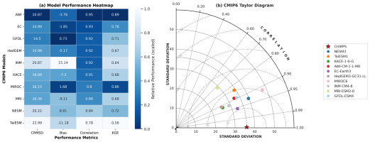
Together, the heatmap and Taylor diagram provide a comprehensive assessment of raw CMIP6 precipitation performance over Sudan. The observed inter-model differences in magnitude, pattern, and combined skill metrics underscore the necessity for bias correction before employing these simulations for impact assessments or climate adaptation planning.
5.2. Bias characteristics
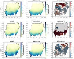
The raw CMIP6 ensemble precipitation over Sudan exhibits substantial annual, seasonal, and spatial biases relative to CHIRPS observations (Fig. 3). At the annual scale (ANN), the median bias is modestly positive at 7.14%, with a wide variability ranging from –82.20% to +100% (standard deviation: 48.01%). Overestimation dominates 60.4% of the country, primarily in the southern regions, while underestimation affects 39.6%, mainly across the northern and western arid zones. This indicates a spatially mixed bias pattern at the annual scale.
Fig. 3.
Seasonal precipitation over Sudan for the annual (ANN), pre-monsoon (March-May; MAM), and monsoon (June-September; JJAS) seasons during 1991-2014. Panels from left to right show CHIRPS observations, raw CMIP6 ensemble mean precipitation, and the corresponding median bias (CMIP6 − CHIRPS) in percent (%). Hatching indicates areas where the bias is statistically significant (p < 0.05), determined using two-sample t-tests.
5.3. Bias correction effectiveness
The performance of four bias-correction techniques: Local Intensity Scaling (LOCI), Delta Change (Delta), Empirical Quantile Mapping (EQM), and Gamma Quantile Mapping (Gamma-QM) was assessed for ten CMIP6 precipitation models over Sudan during 1991-2014, using CHIRPS observations as the reference. Model fidelity was evaluated through Pearson correlation (r), Kling–Gupta Efficiency (KGE), and the centered root-mean-square difference (CRMSD). Figure 4 summarizes inter-model performance across methods. Both EQM and Gamma-QM deliver the strongest and most consistent improvements. Mean correlation (mean ± standard deviation across models) increases from 0.91 ± 0.01 in the raw ensemble to 0.98 ± 0.01 after EQM and 0.98 ± 0.01 after Gamma-QM. Correspondingly, mean CRMSD decreases from 17.7 ± 6.5 mm in the raw simulations to 7.7 ± 0.4 mm (EQM) and 7.9 ± 0.5 mm (Gamma-QM). The average KGE rises sharply from 0.72 ± 0.22 in the uncorrected models to 0.98 ± 0.01 following both quantile-based corrections, indicating a near-complete recovery of observed precipitation variability and bias structure. LOCI yields moderate but robust gains, increasing mean correlation to 0.96 ± 0.01 and KGE to 0.94 ± 0.03, while reducing CRMSD to 9.6 ± 1.1 mm. In contrast, the Delta method exhibits greater inter-model variability, with mean correlation 0.93 ± 0.06, mean KGE 0.91 ± 0.07, and CRMSD 12.7 ± 4.6 mm. Although Delta performs comparably to LOCI for several models, its linear scaling approach fails to capture nonlinear precipitation biases fully, resulting in less uniform improvements.
Fig. 4.
Heatmaps illustrating Pearson correlation coefficient, Centered Root Mean Square Difference (CRMSD), and Kling–Gupta Efficiency (KGE) for ten CMIP6 climate models before and after bias correction by LOCI, Delta, EQM, and Gamma methods. Results are benchmarked against CHIRPS observations over Sudan (annual mean, 1991-2014). Superior performance is indicated by higher correlation and KGE, and lower CRMSD values, with EQM and Gamma methods showing consistently better skill.
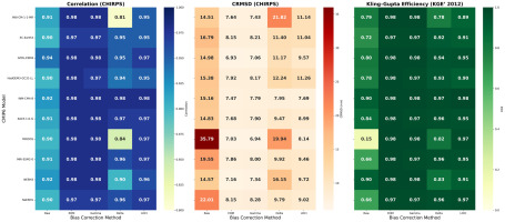
Overall, these results demonstrate that quantile-based bias-correction approaches (EQM and Gamma-QM) are the most effective for CMIP6 precipitation simulations over Sudan. They minimize amplitude errors, enhance temporal coherence with CHIRPS observations, and substantially improve both statistical reliability and physical realism. Such corrections are therefore essential for downstream hydrological and climate-impact analyses in the region.
5.4. Uncertainty assessment via bootstrapping
The robustness of each bias-correction method was evaluated using non-parametric bootstrapping with 1,000 replicates across three seasonal periods: annual, pre-monsoon, and monsoon. Four evaluation metrics were considered: bias, root mean square error (RMSE), Pearson correlation coefficient (r), and Kling– Gupta efficiency (KGE). The corresponding bootstrapped medians with 95% confidence intervals (CIs) are summarized in Table 2.
Table 2.
Bootstrapped (median ±95% CI) evaluation of CMIP6 precipitation over Sudan for Raw and bias-corrected methods (Delta, EQM, Gamma-QM, LOCI) across ANN, MAM, and JJAS periods. Metrics shown include Kling– Gupta Efficiency (KGE), RMSE, Bias, and ΔBias (%), which represents the percentage reduction in absolute bias relative to the Raw simulation.
The bootstrapped results indicate that quantile-based methods (EQM and Gamma-QM) consistently achieve the highest reduction in absolute bias (ΔBias %) across all seasons. For the annual period, EQM achieved the largest improvement with ΔBias = 94%, closely followed by Gamma-QM (ΔBias = 94%). During the pre-monsoon season, both EQM and Gamma-QM fully corrected the mean bias (ΔBias = 100%), reflecting near-perfect alignment with CHIRPS observations. In the monsoon period, Gamma-QM slightly outperformed EQM (ΔBias = 100% vs. 99%), demonstrating robust performance during the main rainy season.
Other methods, such as LOCI and Delta, generally improved model performance but were less consistent. Notably, LOCI slightly increased the absolute bias in the annual period (ΔBias = –13%). Overall, these findings highlight the superiority of EQM and Gamma-QM for correcting precipitation biases in regions with complex seasonal variability, such as Sudan, while simultaneously improving KGE, RMSE, and bias relative to the raw CMIP6 simulations.
5.5. Annual and seasonal evaluation
Figure 5 presents the spatial distribution of seasonal precipitation biases for the ensemble raw and EQM-corrected CMIP6 simulations over Sudan, including maps of bias differences and the statistical significance of the corrections. The raw simulations reveal a mean annual bias close to zero, with a median of 2.16% and substantial spatial heterogeneity (standard deviation: 69.69%). During March-May, biases are dominated by overestimation, with a median of 8.86% and standard deviation of 23.64%, while the June-September period exhibits underestimation, with a median of –6.31% and a standard deviation of 65.22%. Following EQM bias correction, median biases across all seasons are effectively reduced nearly to zero (March-May: –0.21%, June-September: –0.15%, annual: –0.71%), and the spread of residual biases is substantially narrowed (EQM standard deviations: annual 1.01%, March-May 0.43%, June-September 0.71%). The ΔBias (%), representing the relative improvement after EQM correction, shows a median reduction of 96.18% for the annual period, 98.42% for March-May, and 98.75% for June-September, indicating a marked enhancement in model-observation agreement.
Fig. 5.
Spatial distribution of annual and seasonal precipitation biases over Sudan (1991-2014) for the ensemble raw CMIP6 simulations and EQM bias-corrected outputs. Columns represent (from left to right) the raw bias, EQM-corrected bias, and the percentage reduction in bias (ΔBias %) following EQM correction. Units are mm/year for the annual (ANN) row and mm/season for seasonal rows (MAM: March–May, JJAS: June–September). Grey shading in MAM highlights arid northern and central regions with observed precipitation below 10 mm/season, excluded from the ΔBias calculation. Hatching indicates areas where bias reduction is statistically significant (p < 0.05).
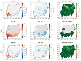
The observed seasonal biases likely arise from a combination of factors inherent to global climate models, including limitations in convective parameterizations, representation of orographic effects, and model resolution constraints, all of which influence the simulation of precipitation intensity and spatial distribution. The pronounced overestimation during the pre-monsoon season may reflect difficulties in simulating the onset of the rainy season, whereas the underestimation during the monsoon season could be related to deficiencies in representing the full intensity and extent of monsoonal rainfall.
While the EQM bias correction method substantially mitigates these systematic biases, it is important to note that bias correction techniques primarily adjust the statistical properties of model outputs and do not address the underlying model physics. Consequently, residual biases and uncertainties may persist, especially under future climate conditions or outside the calibration period. Moreover, the spatial patterns of bias correction effectiveness vary, emphasizing the need for continued model development alongside the application of bias correction approaches.
5.6. Evaluation of model performance
The performance of ten CMIP6 models in reproducing observed precipitation climatology over Sudan was evaluated for annual and seasonal periods. Empirical Quantile Mapping (EQM) was applied to assess its influence on model fidelity. Model skill was quantified using correlation, centered root-mean-square difference expressed as a percentage of observed mean precipitation (CRMSD%) and normalized standard deviation relative to CHIRPS. Both raw and EQM-corrected simulations were analyzed to determine the magnitude of improvement following bias correction.
At the annual scale, EQM substantially reduces model errors, with CRMSD decreases ranging from 35% to 48% compared to the raw simulations (Fig. 6a). EC-Earth3, GFDL-ESM4, and INM-CM4-8 exhibit the strongest improvements, achieving correlations of 0.97 and CRMSD values below 10% of the observed annual mean, indicating a highly realistic representation of spatial rainfall variability.
Fig. 6.
Taylor diagrams for ten CMIP6 models before and after EQM bias correction during (a) annual, (b) March-May, (c) June-September. Each diagram compares model performance with CHIRPS precipitation over Sudan in terms of correlation (radial distance), CRMSD (curved distance from the reference point), and standard deviation (distance from the origin). Star markers denote CHIRPS; circles represent raw models; triangles represent EQM-corrected models.

During the pre-monsoon season, model performance shows greater variability (Fig. 6b). EQM reduces CRMSD for all models, with the best-performing models (NESM3, EC-Earth3, and GFDL-ESM4) achieving CRMSD levels of 12-18% of observed seasonal precipitation and correlations between 0.81 and 0.91. These results highlight the effectiveness of EQM in correcting models that initially underestimated early-season rainfall.
For the main monsoon season, EQM correction again improves simulation fidelity (Fig. 6c). EC-Earth3, GFDL-ESM4, and INM-CM4-8 continue to rank highest, with correlations of 0.87-0.88 and CRMSD values of 15-20% relative to CHIRPS. Although correlations are slightly lower than at the annual scale, these models consistently capture the spatial distribution of monsoon rainfall.
Overall, converting the evaluation to a percentage-based framework demonstrates that EQM significantly enhances CMIP6 precipitation simulations by reducing systematic biases and improving spatial pattern agreement across Sudan’s diverse climatic zones.
Overall, the Taylor diagram analysis (Fig. 6) demonstrates that EQM bias correction substantially improves the statistical agreement of CMIP6 ensemble simulations with observations across all seasons. EC-Earth3, GFDL-ESM4, and INM-CM4-8 are consistently the top performers annually and during the monsoon season, while NESM3 excels during the pre-monsoon season. These results highlight both the effectiveness of statistical bias correction and the relative strengths of individual models in capturing seasonal precipitation dynamics over Sudan.
6. Discussion
The evaluation of CMIP6 precipitation simulations over Sudan reveals substantial variability in model skill, highlighting the challenges of representing rainfall in arid and semi-arid climates. Raw model outputs exhibit systematic biases, often overestimating rainfall during the pre-monsoon season and underestimating it during the main monsoon (Ayugi et al. 2022; Omay et al. 2023). Although annual biases appear smaller on average, they conceal significant spatial heterogeneity, reflecting compensating errors across northern, central, and southern Sudan. These discrepancies indicate that even the latest CMIP6 models struggle to capture convective rainfall initiation, monsoon propagation, and regional orographic influences: issues that have been documented in other CMIP6 evaluation studies (Vogel et al. 2018; Toolan et al. 2025).
Application of bias correction methods markedly improves simulation fidelity, although effectiveness varies by technique and season. Quantile-based approaches consistently produce the largest reductions in bias while improving temporal correlation and overall model performance (Ayugi et al. 2022; Tiku et al. 2025). These methods effectively mitigate seasonal biases during MAM and JJAS, reducing annual biases substantially. In contrast, simpler methods with linear or intensity-scaling assumptions achieve only moderate improvements and fail to capture the nonlinearity of precipitation distributions during early-season rainfall (Switanek et al. 2017). These findings underscore the importance of advanced, distribution-focused bias correction in regions with highly seasonal and spatially variable rainfall.
Spatially explicit analyses further demonstrate that bias correction reduces not only the magnitude of errors but also improves the representation of precipitation variability in regions critical for water resources and agriculture. By excluding arid northern areas with negligible precipitation (<40% of the seasonal mean), and focusing on statistically significant improvements, this study ensures that methodological enhancements are both hydrologically meaningful and regionally robust. Such a spatially refined evaluation represents an advancement over prior studies, which often assess only mean biases without accounting for spatial heterogeneity or significance (Ayugi et al. 2022; Omay et al. 2023).
Finally, integrating bias reduction with rigorous model evaluation helps identify both the most reliable models and the most effective correction methods. This framework demonstrates that even after statistical correction, intrinsic model characteristics continue to influence seasonal performance. By combining bias correction with model skill assessment, this study provides a robust approach for improving precipitation simulations over Sudan and other regions with complex rainfall patterns (Tiku et al. 2025).
7. Conclusions
This study evaluated the performance of multiple bias correction techniques – LOCI, Delta, EQM, and Gamma-QM – in improving CMIP6 precipitation simulations over Sudan for 1991-2014, using CHIRPS observations as the reference. Raw CMIP6 models exhibited systematic spatial biases, primarily linked to misrepresentation of the Intertropical Convergence Zone (ITCZ) and limitations in convective parameterizations.
Among the tested methods, quantile-based approaches (EQM and Gamma-QM) consistently achieved the largest improvements across statistical metrics (correlation, CRMSD, bias, and KGE), reducing mean bias by up to 90 % and enhancing temporal agreement with observations. LOCI and Delta methods provided moderate improvements, largely correcting mean precipitation, but were less effective in capturing distributional variability. Bias correction effectiveness varied seasonally and spatially, performing best in humid southern regions and during the monsoon season, while residual uncertainties persisted in arid northern areas due to low rainfall and observational limitations.
By integrating multi-metric evaluation, robust bootstrapping, and spatially explicit significance testing, this study demonstrates that advanced, distribution-focused bias correction substantially enhances model fidelity, reproducing realistic spatial and temporal variability across annual and seasonal timescales. These findings provide clear guidance for selecting reliable models and appropriate correction techniques in climate impact assessments and water-resource planning.
Future work should extend these approaches to daily-scale analyses, incorporate multi-reference datasets, and explore dynamical downscaling or hybrid correction frameworks to further improve model realism under changing climate conditions, and to assess the persistence of correction effectiveness under non-stationary climates.


