1. Introduction
Evaluating hydro-climatic variability and land-use/land-cover (LULC) changes that alter river basin hydrology is essential for sustainable water resources planning in monsoon-dominated regions such as central India, where seasonal rainfall, reservoir operations, and expanding human demands interact to produce complex hydrological responses (Rickards et al. 2020). There are many medium-sized Indian basins in which the monsoon provides the bulk of annual runoff and where both climate variability and anthropogenic land-use change can quickly alter the water balance and associated ecosystem services (Momblanch et al. 2020). Understanding these coupled drivers is therefore necessary not only to quantify past and present hydrologic alterations but also to develop robust scenarios of future water availability, flood/drought risk, and sediment/nutrient transport under plausible climate and development trajectories (Clark et al. 2016). Physically-based, semi-distributed hydrological models such as the Soil and Water Assessment Tool (SWAT) have become the workhorse for such basin-scale assessments because they mechanistically link weather, soils, land cover, and management practices to runoff, evapotranspiration, groundwater recharge, and sediment dynamics features that are critical when evaluating the relative contributions of hydro-climatic variability and LULC change to observed hydrological trends (Tena et al. 2019). The SWAT framework explicitly represents the water balance by partitioning precipitation into surface runoff, evapotranspiration, percolation, return flows, and groundwater contributions, which allows researchers to separate the roles of changing rainfall patterns versus changing land surface characteristics on streamflow magnitude and seasonality (Banton et al. 2022). SWAT has been used to quantify historical water yields, investigate sediment sources, and project hydrological responses to climate scenarios (Pathak et al. 2019). The sensitivity of model outputs to key parameters such as the curve number (CN2) and groundwater routing schemes requires careful bias-correction and downscaling of global and regional climate projections for scenario analyses (Feng et al. 2023). For the Tawa basin specifically, remote sensing and GIS-based LULC analyses reveal notable changes over recent decades, including shifts between forest, agricultural land, and range/settlement classes that alter infiltration, surface roughness, and evapotranspiration patterns and thus have the potential to substantially influence runoff and sediment yield (Stecher et al. 2023). Hydrochemical and hydrogeological investigations further indicate that while the basin’s silicate lithology influences base water chemistry, anthropogenic activities, including land clearing, agriculture, and mining, have measurable effects on water quality and likely on the land-surface processes that control hydrological responses during different seasons (Huang et al. 2014). These combined lines of evidence motivate an integrated SWAT-based analysis for the Tawa River basin that explicitly accounts for historical LULC transitions (derived from multi-temporal Landsat and other remote sensing products) together with observed hydro-meteorological variability, and that evaluates model sensitivity and uncertainty using recommended calibration and validation frameworks (Pai, Saraswat 2013). Methodologically, such an approach typically begins with high-quality geospatial inputs (DEM, soil maps, and LULC layers), station or gridded weather data for the historical baseline, and an HRU (hydrological response unit) delineation strategy that balances physical realism and computational tractability. Calibration is then conducted against streamflow (and where available, sediment) records using automated/semi-automated tools (e.g., SWAT-CUP and SUFI-2) to estimate parameter ranges and predictive uncertainty (Corona et al. 2014; Rickards et al. 2020). Once validated, scenario experiments can isolate LULC versus climate influences by holding one driver constant while perturbing the other, for example, running the model with historical climate but with a sequence of synthetic or observed land-cover maps to quantify the hydrologic imprint of land conversion, and conversely, simulating evolving climate forcing under constant LULC to quantify hydro-climatic impacts (Sidău et al. 2021).
The present study provides a comprehensive assessment of how hydro-climatic variability and LULC change have jointly altered the hydrological behavior of the Tawa River basin. The observed increase in monsoonal rainfall, as identified through trend analysis, has directly influenced annual water availability; however, its hydrological benefits are not uniformly translated into sustainable streamflow because of concurrent land transformation. The expansion of agricultural and urban areas at the expense of forest and rangeland has emerged as a dominant driver of hydrological change in the basin. Forested landscapes typically enhance infiltration, delay runoff, and sustain base flow through gradual groundwater release. Their reduction has resulted in increased surface runoff and reduced subsurface flows, as reflected in declining base flow and groundwater recharge simulated by the SWAT model. Similar hydrological responses have been reported in other central Indian basins, where deforestation and agricultural intensification have amplified runoff coefficients and reduced dry season flows. The increasing dominance of surface runoff during the monsoon season suggests a heightened vulnerability to flood events, particularly under projected increases in rainfall intensity associated with climate change. At the same time, reduced base flow during post-monsoon and dry periods may intensify water scarcity for irrigation and ecological needs. This seasonal imbalance underscores the importance of analyzing not only total water yield but also flow partitioning when assessing basin-scale hydrological impacts. Rising temperatures and modified cropping patterns have contributed to increased evapotranspiration, partially offsetting gains in rainfall-induced water yield. This finding highlights the complex, non-linear interactions between climate variables and land surface processes. Although climate variability governs interannual fluctuations in hydrological components, land-use change exerts a more persistent, structural control over runoff generation and groundwater recharge.
From a management perspective, the results emphasize the need for integrated land and water resource planning in the Tawa River basin. Strategies such as afforestation, conservation agriculture, and protection of recharge zones could help restore hydrological balance and enhance climate resilience. The modeling framework adopted in this study offers a transferable approach for evaluating hydrological responses in other data-scarce, monsoon-driven river basins.
2. Study area description
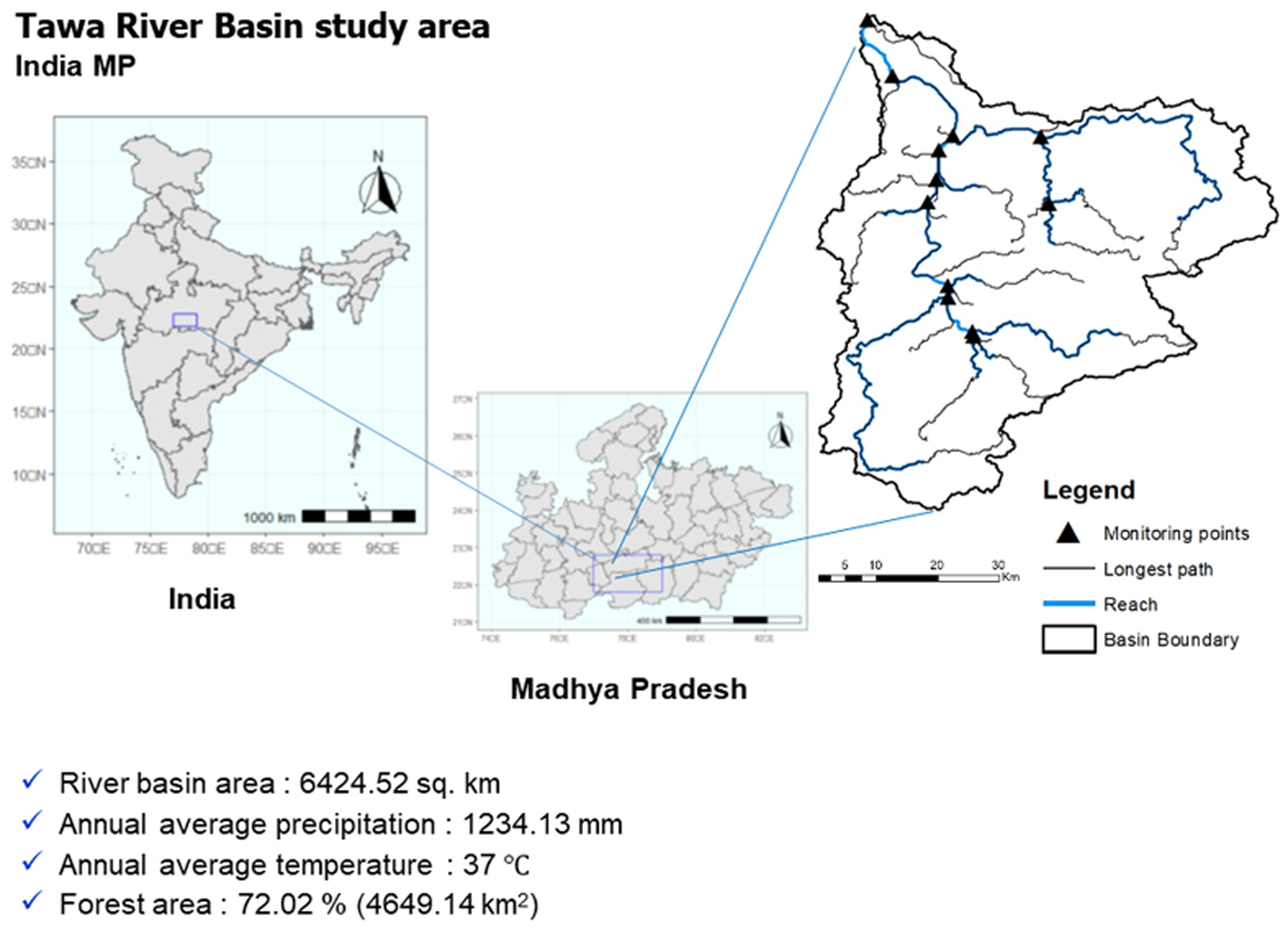
The Tawa River basin, the focus of this study (Fig. 1), spans 6424.52 km2 and includes parts of several districts and tehsils (Nema et al. 2016). In Hoshangabad district, it covers the Hoshangabad and Sohagpur tehsils; in Betul district, it includes the Betul and Multai tehsils, and in Chhindwara district, it encompasses the Tamia and Jamai tehsils (Rajput et al. 2021). The study area is located between latitudes 21°45' and 22°50' and longitudes 77°40' and 78°45'. It lies within Survey of India degree sheets 55F, 55G, 55J, and 55K at a scale of 1:250,000, as well as parts of Survey of India topo sheets at a scale of 1:50,000. The plains of the valley are occasionally interrupted by isolated knolls and stony ranges, providing relief from the flatlands (Sridhar, Chamyal 2010). The hills in the region are part of the northern Mahadeva hill ranges of the Satpura Mountains, stretching in an east-west direction. Notable hills include Motur, Kalapahar, and Dulhadeo, with altitudes ranging from 321 to 1304 m above mean sea level (Kathal 2018). The Narmada River flows along the northern edge of the valley near Jabalpur, traversing alluvial basins interspersed with rocky gorges. Moving westward for 350 km across alluvial plains south of the valley, it passes beyond Handia, meanders through forested hills, and becomes visible again near Mandhata, entering the Mandleshwar Plain, a 150 km stretch of alluvium (Rajaguru et al. 1995), where the river valley transforms into an estuary, extending for 25 km as the Narmada enters the Gulf of Cambay (Saraswat, Solanki 2021). The Narmada River is fed by several major tributaries, including Tawa, Karanj, Goi, and Gujal on its southern bank, and Hiran, Hatni, Man, and Kanar on its northern bank (Gupta, Chakrapani 2005).
3. Data and methods
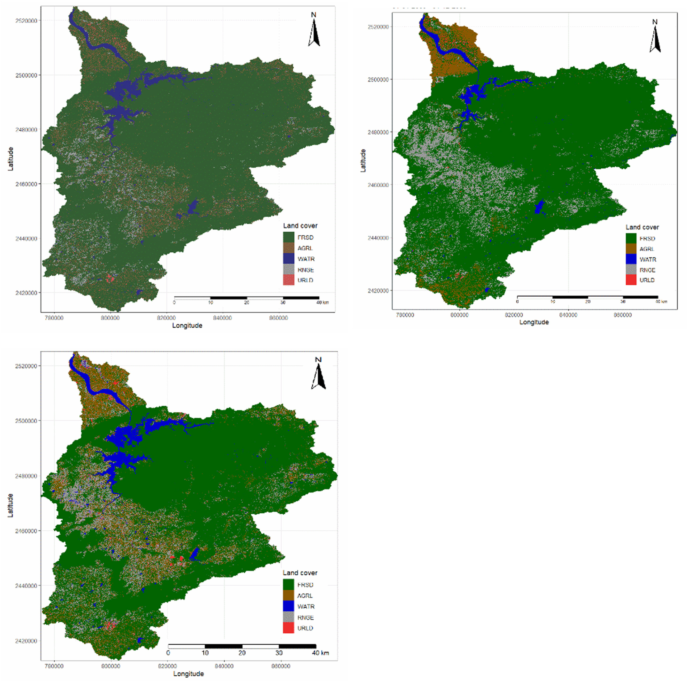
We have used gauge station-based discharge data, simulated and observed climate model products, gridded observed meteorological data, and LULC (Fig. 5) derived from Landsat satellite images and other auxiliary data sets (soil type and topography). Table 1 provides a detailed description of the data sets used. In this study, a combination of gauge-based hydrological observations, gridded meteorological products, satellite-derived land surface information, and ancillary geospatial datasets was employed to ensure a comprehensive representation of hydro-climatic processes within the basin. Daily rainfall and minimum/ maximum temperature records were derived from the India Meteorological Department (IMD). These data are widely recognized for their reliability in hydrological and climate impact assessments across India. These data sets formed the primary climatic drivers for the Soil and Water Assessment Tool (SWAT) simulations. Land use and land cover (LULC) information, a critical determinant of surface hydrology, was extracted from multi-temporal Landsat satellite images (Fig. 2).
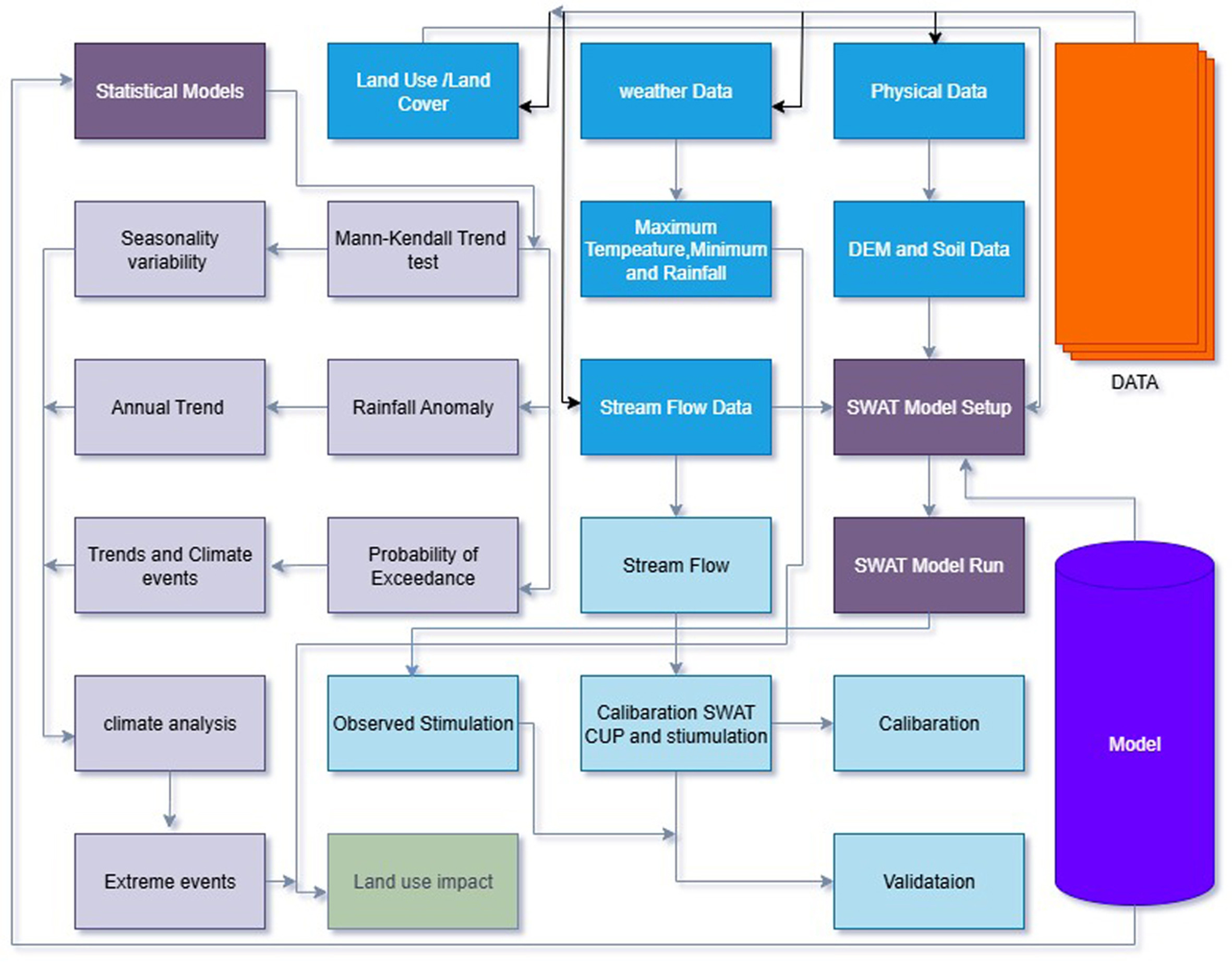
Table 1.
Details of the datasets used in this study.
| Input data type | Parameter | Source | Resolution | |
|---|---|---|---|---|
| Physical data | Topography | SRTM Digital Elevation Model (DEM) (http://earthexplorer.usgs.gov/) | 30 m | |
| Land use | Landsat 5, 7, and 8 (http://earthexplorer.usgs.gov/) | 30 m | ||
| Soil-type | Food and Agriculture Organization of the United Nations (FAO) (https://www.fao.org/ ) | 500 m | ||
| Meteorological data (historical) | (rainfall and min-max temperature) | India Meteorological Department (IMD) (https://www.imdpune.gov.in) | 0.25° × 0.25° and 1° × 1° | |
| Observed hydrological data | Gauge data (river discharge) | Central Water Commission (CWC), India (http://www.cwc.gov.in/ ) | Daily | |
| Soil Water Assessment Tool (SWAT) | - | https://swat.tamu.edu/ | - | |
3.1. Hydro-climatic data
Increasing temperature in semi-arid areas like the Tawa River basin mostly enhances evaporation and therefore, changes in climate influence river discharge. For this study, we have used IMD meteorological data. The observed rainfall and temperature (minimum and maximum) data, with spatial resolutions of .25° × .25° and 1° × 1°, were derived from IMD meteorological data from 1999 to 2019.
3.2. Land use and land cover mapping
The maximum likelihood classification (MLC) algorithm of the supervised classification technique has been applied to Landsat images (05, 07, and 08) from 1999, 2009, and 2019 (pre-monsoon seasons) to obtain LULC for the entire study area. The modified classification scheme of the National Remote Sensing Agency (NRSC), India and the Anderson classification system (Anderson et al. 1976) were selected to classify the study area into seven different LULC classes, namely: built-up land, agriculture land, water bodies, barren land, shrub land, open forest, and dense forest. The Land Change Modeler (LCM), integrated software developed by IDRISI Selva (Eastman 2016), has been used for analyzing and predicting LULC changes in the basin. Other details pertinent to the LULC of the entire study area are available in Patil et al. (2025).
3.3. Soil and Water Assessment Tool (SWAT)
SWAT is a conceptual, semi-distributed, time-continuous, physically based, comprehensive, process-oriented, watershed-scale model that was initially developed by the United States Department of Agriculture (USDA) Research Service and Texas A&M University (Arnold et al. 1998; 2012) to understand the dynamics of hydrological systems. It simulates water cycle components as well as the effects of management practices on fluxes of energy and matter at daily time steps, but can aggregate the results to monthly or annual output (Arnold et al. 1998; 2012). SWAT lumps areas having homogeneous soil, topography, management, and land use characteristics into unique hydrologic response units (HRUs) within the sub-watersheds of a basin. These HRUs have no interconnection among them and are routed individually following the law of water balance toward the outlet of the sub-basins (Arnold et al. 1998; Neitsch et al. 2011). The SWAT model computes surface runoff based on the Soil Conservation Services (SCS) curve number method (Anand, Rajaram 2004). A detailed description of the SWAT model and its components is available at (https://swat.tamu.edu).
3.3.1. SWAT model setup and evaluation criteria
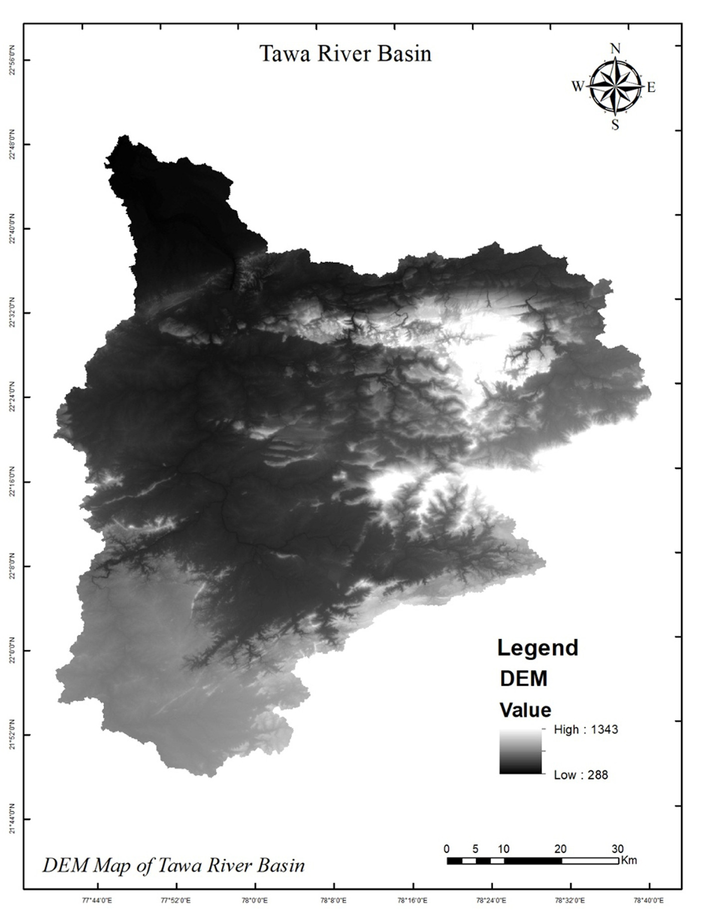
The SWAT model has been set up to simulate hydrological responses of the Tawa River basin toward ongoing LULC and climate changes. The SWAT model was provided with the required input data, viz., soil (Fig. 3), land use (Fig. 5) for 2019, elevation (DEM) (Fig.4), and meteorological data in the desired format to simulate streamflow at the outlet of the Tawa River basin. In order to simulate the historical streamflow under the synergistic effects of LULC and climate change, the SWAT model was set up for the observed time periods of 20 years (1999 to 2019), including three years as a warm-up period with land use imagery from 2019. The R 2 statistic indicates the proportion of the variance (relative to the mean) in the observed data; its value varies from 0 to 1, where values closer to 1 indicate better model simulations. The NSE is a dimensionless normalized statistic that determines the relative magnitude of the residual variance (noise) compared to the measured data variance (information) (Nash, Sutcliffe 1970). The NSE value ranges from ∞ to 1, where a value close to 1 indicates a perfect fit. It is sensitive to differences in the observed and model-simulated means and variances. The PBIAS measures the average tendency of the simulated data to be larger or smaller than their observed counterparts (Gupta et al. 1999).
3.3.2. Computation modeling
In hydrological modeling, calibration and validation are essential to ensure that the model accurately simulates observed streamflow and other hydrological variables. The Soil and Water Assessment Tool (SWAT) employs statistical performance metrics to evaluate the agreement between simulated and observed data during both calibration and validation phases. The most widely used statistical indicators include the Nash–Sutcliffe Efficiency (NSE), Coefficient of Determination (R2), and Percent Bias (PBIAS).
• Nash–Sutcliffe Efficiency (NSE)
The NSE measures the predictive power of the model by comparing observed and simulated values:
where: Qobs,i – observed streamflow at time i; Qsim,i – simulated streamflow at time I;
The NSE ranges from −∞ to 1, with values closer to 1 indicating better model performance (Nash, Sutcliffe 1970).
• Coefficient of Determination (R2)
R2 quantifies the proportion of variance in the observed data that is explained by the simulated data:
where:
R2 values range from 0 to 1, with values closer to 1 indicating strong correlation (Krause et al. 2005).
• Percent Bias (PBIAS)
PBIAS measures the average tendency of simulated values to be larger or smaller than observed values:
Positive PBIAS values indicate model underestimation, while negative values indicate overestimation (Gupta et al. 1999).
• Root Mean Square Error–Observation Standard Deviation Ratio (RSR)
where: standardized RMSE by dividing by the standard deviation of observed data. RSR values close to 0 indicate better model performance.
3.3.3. Trend analysis
• Mann–Kendall Trend Test
The Mann–Kendall (MK) test is a non-parametric statistical test widely used to detect monotonic trends in hydrological and climatological time series without requiring the data to follow a specific distribution.
Equation for the test statistic:
where xi and xj are data values at times i and j; n is the number of observations.
Variance (for no ties):
• Rainfall anomaly
Rainfall anomaly quantifies the deviation of annual or seasonal rainfall from its long-term mean, expressed either in absolute or percentage form.
where: Pi – rainfall in year i;
A positive anomaly indicates wetter-than-average conditions; a negative anomaly indicates drier-than-average conditions.
• Probability of exceedance
The probability of exceedance (Pe) represents the likelihood that a rainfall event of a given magnitude will be equaled or exceeded in any given year.
where: m – rank of the rainfall event (largest = 1, smallest = n); n – total number of years of record.
Alternatively, the Return Period (T) is related to exceedance probability by:
• Coefficient of Variation (CV)
The Coefficient of Variation (CV) is a statistical measure used to quantify the relative variability of a dataset with respect to its mean. It provides a standardized measure of dispersion, allowing comparison of variability among hydro climatic variables with different units or magnitudes. The CV is calculated as:
Where CV represents the coefficient of variation, σ denotes the standard deviation, and X represents the long-term mean of rainfall, temperature, and streamflow. A low CV indicates that the data points are closely clustered around the mean, reflecting low variability. In contrast, a high CV value suggests greater dispersion of observations relative to the mean, indicating higher variability. In this study, the inter-annual variability of hydro climatic variables was assessed using CV and categorized as follows: low variability (CV < 20%), moderate variability (20% ≤ CV < 30%), high variability (30% ≤ CV < 40%), very high variability (40% ≤ CV < 70%), and extremely high variability (CV ≥ 70%). This classification framework was used to evaluate the degree of variability in rainfall, temperature, and streamflow across the study period.
• Standard Anomaly Index (SAI )
The Standard Anomaly Index (SAI )is a statistical indicator used to quantify the deviation of an individual observation from the long-term mean of a dataset. It is particularly useful for identifying wet and dry years in hydro-climatic time series such as rainfall, temperature, and streamflow, and for examining temporal trends (Alashan 2020).
The SAI is computed as:
where: SAI is the Standard Anomaly Index, X is the individual observation, x is the long-term mean, and σ is the standard deviation of the dataset.
The SAI expresses deviations in standardized units, enabling comparison across variables and time periods. A positive SAI value indicates that the observation is above the long-term mean, representing a relatively wet (or above-average) condition. Conversely, a negative SAI value indicates below-average conditions, corresponding to relatively dry periods. The classification of SAI values into wetness and dryness categories is presented in Table 2.
Table 2.
Classification of Standard Anomaly Index (SAI) values.
3.4. Soil data
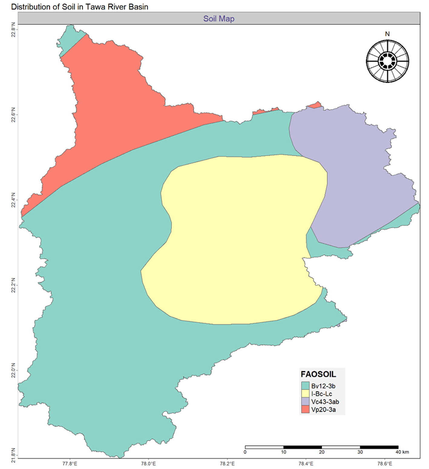
Soil information for the Tawa River basin was obtained from the Food and Agriculture Organization (FAO) digital soil database. The FAO soil map was extracted and clipped to the basin boundary using GIS techniques, and soil mapping units were reclassified according to FAO soil taxonomy. The dominant soil units identified within the basin include Bv12-3b, I-Bc-Lc, Vc43-3ab, and Vp20-3a. Among these, Bv12-3b (Vertisols) occupies the largest spatial extent, particularly across the central and southern parts of the basin, followed by Vc43-3ab and I-Bc-Lc units, while Vp20-3a is distributed in smaller localized patches. These soils are predominantly clay-rich with moderate to high water-holding capacity and varying infiltration characteristics. The spatial soil layer was converted into raster format and integrated into the SWAT model for hydrological simulation. Soil physical properties, including texture, hydraulic conductivity, bulk density, and available water capacity, were assigned based on FAO database attributes and supplemented with literature values where necessary. The processed soil dataset was subsequently combined with LULC and digital elevation model (DEM) data to delineate Hydrological Response Units (HRUs), ensuring accurate representation of soil–land use interactions in runoff and groundwater recharge simulations.
3.5. Model calibration, validation, and performance evaluation
The accuracy with which a hydrological model is calibrated determines its efficiency. The calibration, validation, and sensitivity analysis of the SWAT model were performed monthly using recently developed SWAT-Calibration and Uncertainty Programs (SWAT-CUP). SWAT-CUP is a Sequential Uncertainty Fitting version 2 (SUFI2) algorithm-based hydrological parameter sensitivity and uncertainty analysis framework (Abbaspour et al. 2007). The SUFI-2 incorporates Latin hypercube (LH) techniques that facilitate a time-variable approach to ascertain the most sensitive parameters. A set of sensitive parameters was used for manual calibration and validation of the SWAT model. SUFI-2 supports access to the quantitative statistical procedures, namely NSE, PBIAS, R 2, and RSR (Moriasi et al. 2007) for evaluation of overall model performance (Table 3).
Table 3.
Recommended statistical standard of model performance rating for a monthly time-step by Moriasi et al. (2007).
4. Result and analysis
4.1. SWAT model sensitivity and performance
The SWAT-CUP-based SWAT model calibration was carried out using 14 parameters (CN2, ALPHA_BF, GWQMN, ESCO, CH_K2, CH_N2, REVAPMN, SOL_AWC, HRU_SLP, SOL_BD, SLSUBBSN, GW_REVAP, GW_DELAY, SURLAG, and OV_N) at a monthly time step. Observed daily discharge data obtained from the Central Water Commission (CWC), India, were used from 1986-1995 for calibration and from 1998-2002 for validation. The discharge records were collected from the Hoshangabad gauging station of CWC, India, located at the outlet of the Tawa River Basin. Model performance during the calibration and validation periods yielded NSE, PBIAS, R2, and RSR values of 0.66, –9.1, 0.67, and 0.58, and 0.64, 8.1, 0.65, and 0.60, respectively. Based on the performance criteria recommended by Moriasi et al. (2007), the SWAT-CUP-based model performance was categorized as “Good” for calibration (Fig. 6) and Satisfactory for validation (Fig. 7). According to Abbaspour et al. (2007), parameters with higher t-statistic values and lower p-values are considered more sensitive. Among the calibrated parameters, ALPHA_BF was identified as the most sensitive, followed by SLSUBBSN and SOL_AWC. Overall, the model output showed sensitivity to all 14 parameters listed in Table 4. The calibrated and validated SWAT model was subsequently applied to simulate streamflow in the Tawa basin under different LULC and climate scenarios.
Fig. 6.
Shows 95PPU (the region of lower uncertainty) graph of calibration, performed on SWAT-CUP using monthly simulated and observed discharge data at the outlet of the Tawa River basin.
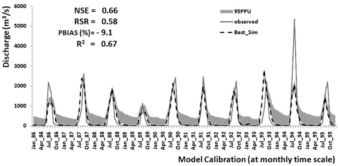
Fig. 7.
Shows 95PPU (the region of lower uncertainty) graph of validation, performed on SWAT-CUP using monthly simulated and observed discharge data at the outlet of the Tawa River basin.
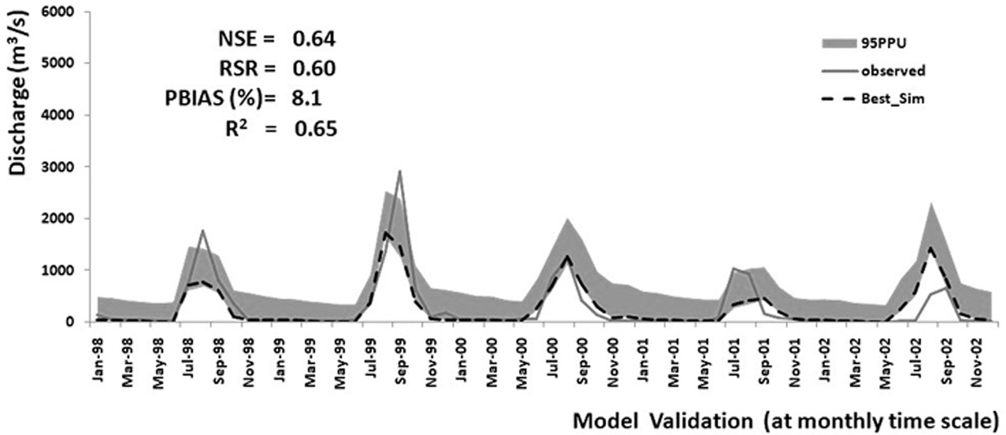
Table 4.
Summary of sensitive SWAT parameters with their corresponding maximum and minimum values.
4.2. Hydrological response
The hydrological response of the Tawa River basin to hydro-climatic variability and LULC change was analyzed using SWAT-simulated components, including surface runoff, base flow, evapotranspiration, groundwater recharge, and total water yield. The calibrated model adequately captured the observed streamflow dynamics, with performance statistics indicating satisfactory to good agreement between simulated and observed flows (NSE > 0.65, R2 > 0.70, and PBIAS within ±15%). The simulation results show a clear increase in surface runoff over the study period, particularly during the monsoon season. This increase is closely associated with the expansion of agricultural and urban land and the corresponding reduction in forest and rangeland areas, which has decreased infiltration capacity and increased overland flow. Seasonal analysis indicates that peak flows have become more pronounced, suggesting a higher risk of flash floods under extreme rainfall events. In contrast, groundwater recharge and base flow contributions to total streamflow exhibit a declining trend. The reduction in forest cover and increased soil compaction in agricultural areas have limited percolation to deeper soil layers, thereby reducing subsurface flow contributions during the post-monsoon and dry seasons. As a result, lean-season flows have diminished, potentially affecting irrigation and ecological water requirements. Evapotranspiration shows a moderate increase, driven by rising temperatures and changes in cropping patterns. Although increased rainfall has enhanced overall water yield, its benefits are partly offset by higher evapotranspiration losses and altered flow partitioning. Scenario-based simulations further reveal that LULC change exerts a stronger influence on runoff generation and base flow reduction, whereas climate variability primarily controls interannual variability in total water yield. These findings highlight the nonlinear and compounded effects of climatic and anthropogenic drivers on basin hydrology.
4.3. Land use/land cover changes
Five major LULC types: forest, agriculture, water bodies, rangeland, and urban land were classified for the years 1999, 2009, and 2019 (Table 5). The results indicate that the total geographical area of the Tawa River basin is 6,455.33 km2. The spatial extent and percentage share of each LULC class for the three study periods are summarized in Table 5. The LULC classification of the Landsat TM 1999 image reveals that the basin was predominantly occupied by forest and agricultural land, jointly covering approximately 5,886.73 km2 (91.9%) of the total area. Forest cover alone accounted for 5,333.99 km2 (82.63%), while agricultural land covered 552.75 km2 (8.56%). Urban land and water bodies occupied relatively smaller areas of 41.92 km2 (0.65%) and 257.45 km2 (3.99%), respectively (Fig. 3). Rangeland covered 269.23 km2 (4.17%) of the basin. Similarly, in 2009, forest and agricultural land together constituted the largest share of the basin, covering 5,572.56 km2 (86.32%). Forest area slightly declined to 5,258.10 km2 (81.45%), while agricultural land reduced to 314.47 km2 (4.87%). Urban land and water bodies covered 49.63 km2 (0.77%) and 265.45 km2 (2.11%), respectively (Fig. 5). In contrast, rangeland showed a substantial increase, occupying 696.69 km2 (10.79%) of the basin. The LULC classification of the Landsat OLI 2019 image also indicates that forest and agriculture remained the dominant land cover types, together accounting for 5,438.47 km2 (84.25%) of the total basin area. Forest cover declined markedly to 4,649.15 km2 (72.02%), while agricultural land expanded to 789.32 km2 (12.23%). Urban land and water bodies increased to 59.09 km2 (0.92%) and 276.56 km2 (4.28%), respectively (Fig. 5). Rangeland covered 681.22 km2 (10.55%) of the basin. Although forest and agricultural land continued to dominate the basin in 2019, the forest cover experienced an overall decline of approximately 10% between 1999 and 2019, indicating significant conversion of forest areas into agricultural land and urban settlements. Forest remains the principal land cover in the Tawa River basin and plays a crucial role in maintaining ecosystem functions and regulating climatic processes from the local to the regional scale.
Table 5.
Area of LULC classes 1999, 2009, and 2019.
4.4. Hydro-climatic trend analysis
4.4.1. Time series analysis of annual precipitation and temperature
Rainfall is a complex natural hydrological phenomenon that has a direct impact on the hydrology of the land surface. The observed average annual rainfall (mm) data from the Tawa River basin for the baseline period of 1981 to 2020 over the entire basin shows, to some degree, a declining trend. The calibrated and validated SWAT model has been used for assessing the effects of LULC and climate change on streamflow under the baseline climate scenario in the Tawa River Basin (Fig. 8). Maximum rainfall was observed in 2006, 2013, 2016, and 2019. The average annual precipitation during the baseline period varied between 2.41 and 5.09 mm. The average annual precipitation over the Tawa River Basin showed an increasing trend during the baseline period. The analysis of annual precipitation trends from 1999 to 2020, as depicted in the accompanying graph, offers valuable insights into climatic patterns over the two-decade period. The graph illustrates annual precipitation levels (in mm) plotted against the years, with a fitted linear regression line (y = 0.0329x – 61.732) and a coefficient of determination (R2 = 0.2182).
Fig. 8.
Variation in average annual precipitation over the Tawa River basin n during the baseline period.
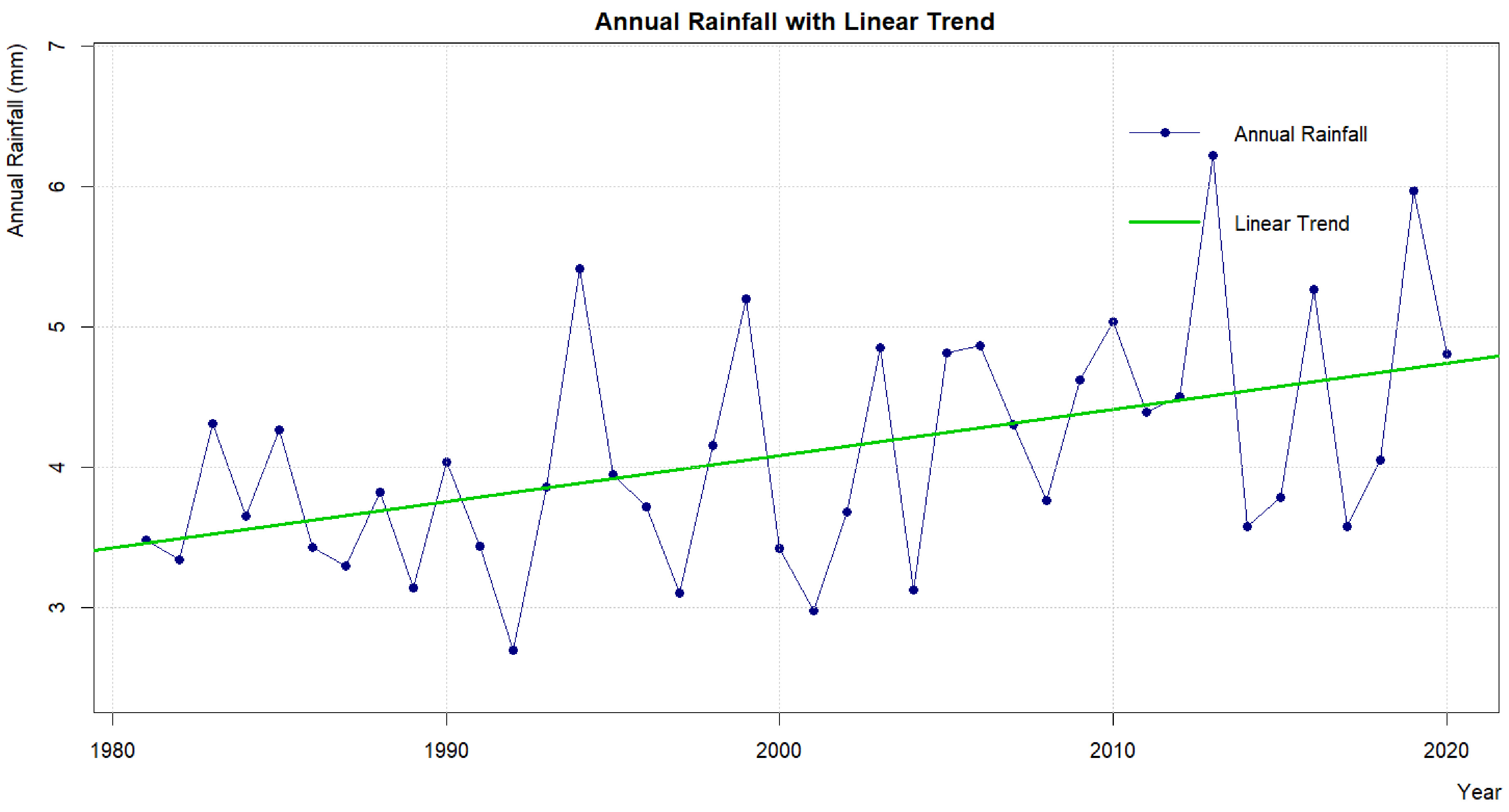
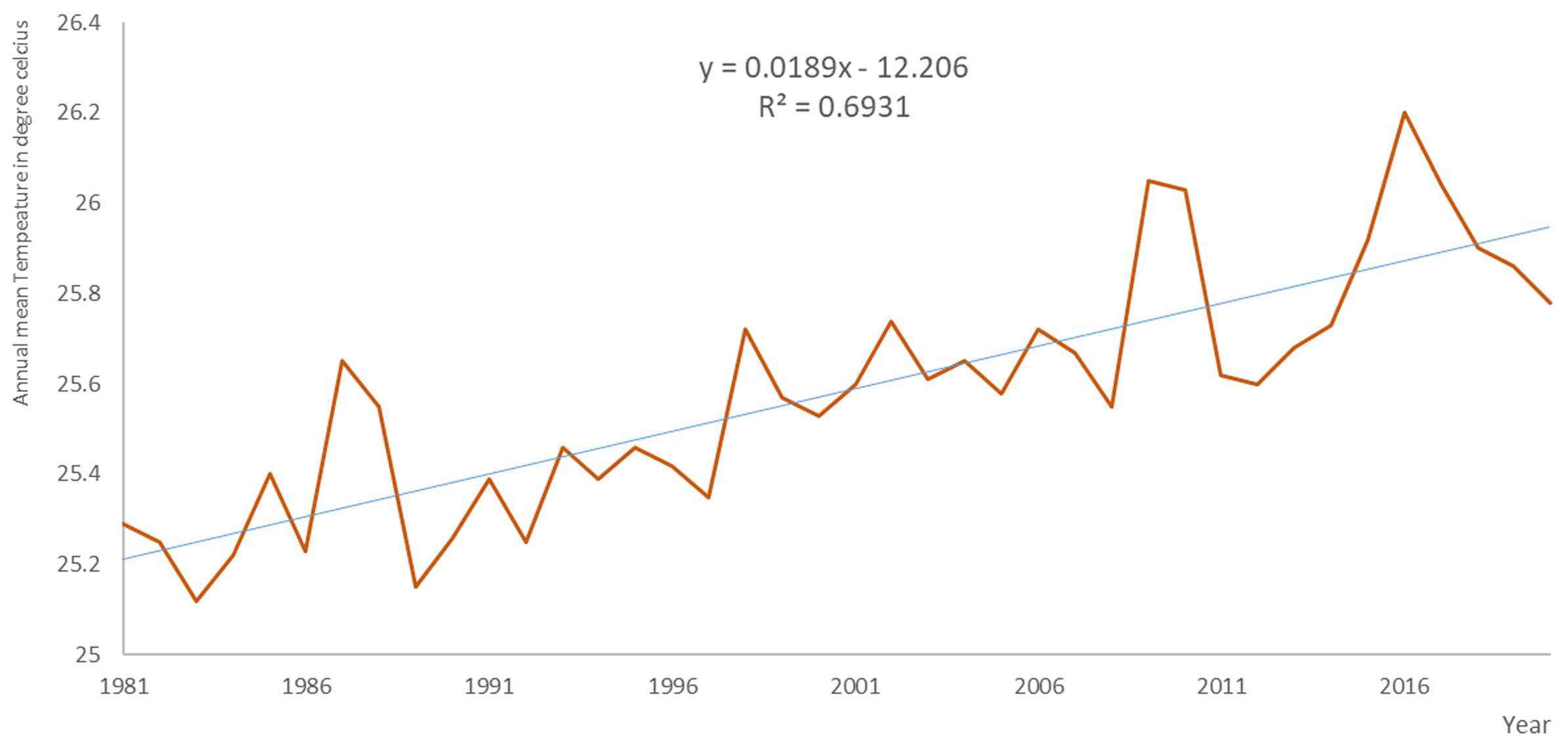
This study aims to interpret these data to understand long-term precipitation behavior and its implications. The data reveal a slight upward trend in annual precipitation, as indicated by the positive slope of the regression line. Starting at approximately 3 mm in 1999, the average precipitation shows a gradual increase, reaching around 4 mm by 2020. The regression equation suggests an average increase of 0.0224 mm per year, though the low R2 value (0.0376) indicates that only about 3.76% of the variability in precipitation can be explained by the linear model. This suggests that while there is a general upward trend, year-to-year fluctuations dominate the dataset, reflecting the inherent variability of climatic systems. Figure 9 represents climate change; from 1999 to 2005, the average annual minimum temperature at the outlet point of the basin remained relatively steady, hovering around 19°C. This period can be characterized by consistent, normal temperature levels, with little variation observed in the data. In contrast, from 2006 to 2019, the average annual minimum temperature increased slightly to approximately 20°C.
4.4.2. Mann-Kendall trend test and trend
The Mann-Kendall trend test was applied to a 40-year annual rainfall time series from the Tawa River basin in central India. The test yields a standardized statistic of Z = 2.6448 and a p-value of 0.008174, which falls well below the 0.05 and 0.01 significance levels, thereby rejecting the null hypothesis of no trend at high confidence. The positive Z -value indicates an increasing direction in annual rainfall totals, while Kendall’s tau of 0.2923 denotes a moderate positive monotonic association between time and rainfall, situated at the interface of weak-to-moderate strength and reflecting a consistent tendency toward higher precipitation amid interannual variability. The computed Mann-Kendall S-statistic of 228 (with variance 7366.67) further corroborates this non-random upward pattern across the ranked pairwise comparisons. This observed increasing trend in annual rainfall aligns with emerging evidence from hydrological and climatological investigations in the Tawa basin and broader central Indian regions. However, prior analyses of seasonal rainfall in the Tawa Basin area and adjacent parts of Madhya Pradesh have occasionally reported insignificant or decreasing trends in mean annual or monsoon precipitation over certain historical periods, highlighting spatial heterogeneity and the influence of multi-decadal variability. The current finding of a significant positive trend over the 40-year record may indicate a shift toward wetter conditions in this sub-basin, potentially linked to regional climate dynamics, including altered monsoon moisture convergence under global warming influences. This analysis has benefited from the robustness of the non-parametric Mann-Kendall approach, which is well-suited to non-normally distributed hydrological data. In conclusion, the statistically significant increasing trend in annual rainfall detected herein underscores a potentially favorable shift in hydroclimatic conditions within the Tawa River basin, with implications for enhanced surface water availability, agricultural productivity in the irrigated command area, reservoir operations (e.g., Tawa Dam), and flood risk management. Nevertheless, given the basin's vulnerability to intra-seasonal extremes and broader uncertainties in climate projections for central India, adaptive water resource strategies remain essential to ensure sustainable utilization amid ongoing environmental changes.
4.4.3. Rainfall anomaly and variability analysis
The Mann-Kendall trend test, applied to the 40-year (1981-2020) annual rainfall time series from the Tawa River basin, a key sub-basin of the Narmada River system in central India, across parts of Madhya Pradesh, indicates a statistically significant upward monotonic trend. The test produces a standardized Z-statistic of 2.6448 and a p-value of 0.008174, which is substantially below the 0.05 and 0.01 significance thresholds, thereby providing strong evidence to reject the null hypothesis of no monotonic trend. The positive sign of Z confirms an increasing direction in annual rainfall totals, while Kendall’s tau of 0.2923 signifies a moderate positive monotonic association between time and rainfall amounts, positioned at the weak-to-moderate strength boundary and indicative of a consistent long-term tendency toward higher precipitation despite considerable interannual fluctuations.
Examination of the time series data reveals pronounced variability, with annual rainfall ranging from a low of approximately 2.70 units (likely in thousands of mm or normalized units; 1992) to a high of 6.22 units (2013), accompanied by large anomalies and Standardized Anomaly Index (SAI ) values. Notably, extreme wet years are evident in 2013 (anomaly +2.12, SAI +2.58), 2019 (anomaly +1.87, SAI +2.27), 1994 (anomaly +1.32, SAI +1.60), and 2016 (anomaly +1.17, SAI +1.42), while severe dry conditions occurred in 1992 (anomaly –1.40, SAI –1.70), 2001 (anomaly –1.12, SAI –1.36), and 1989 (anomaly –0.96, SAI – 1.16). The CV remains constant at approximately 20.1% across the period, reflecting moderate-to-high interannual variability typical of monsoon-dominated regimes in central India. The increasing trend appears driven in part by a clustering of above-average years in the later portion of the record (e.g., post-2005, with several SAI values exceeding +0.8 and peaks in the 2010s), suggesting a possible shift toward wetter conditions in recent decades (Fig. 10 and 11).


This detected positive trend in annual rainfall is broadly consistent with regional hydroclimatic patterns observed in parts of the basin and central India, where some studies have documented enhancements in monsoon precipitation intensity or total accumulation under the influence of global warming, altered atmospheric circulation, and increased moisture convergence during the southwest monsoon season. However, rainfall trends in this region exhibit considerable spatial and temporal heterogeneity. Some analyses of adjacent areas or seasonal components (e.g., monsoon months) have reported insignificant, stationary, or even declining tendencies over overlapping or differing periods.
In conclusion, the statistically significant increasing trend in annual rainfall over the 1981-2020 period points to an emerging hydroclimatic shift toward greater water availability in the Tawa River basin. This finding has potential positive implications for rainfed and irrigated agriculture in the Tawa command area, reservoir inflow and storage dynamics at Tawa Dam, and overall basin water security. Nonetheless, the high interannual variability (CV ≈ 20%) and the risk of extreme wet and dry years necessitate continued monitoring, incorporation of climate model projections (e.g., under CMIP6 scenarios), and adaptive management strategies to mitigate flood risks during intense monsoon episodes while optimizing resource use during drier intervals amid broader uncertainties in regional climate change.
4.4.4. Estimation of the probability of exceedance
The frequency analysis and return period assessment of annual precipitation (PRCP) in the Tawa River basin, based on a 45-year record (approximately 1981-2025, with 2024 and 2025 included as recent or provisional values), reveal important insights into the distribution of rainfall extremes and recurrence intervals (Fig. 12). The table ranks annual PRCP values in descending order, from the highest recorded year (2007: 171.35 units, likely mm or a standardized basin-average) with a rank of 1 and an exceedance probability Fa of 0.68% (corresponding to a return period T ~ 148 years), to lower values such as 2006 (32.04 units, rank 45, Fa ~ 60.14%, T ~ 1.66 years). The exceedance probability Fa is calculated as (rank/(n + 1)) × 100%, where n = 45 (or adjusted for plotting position formula), and the return period T is estimated as 1/(Fa/100), representing the average recurrence interval for events exceeding the given PRCP threshold (Table 6).
Table 6.
Estimated probabilities of exceedance of the ranked annual rainfall.
The results highlight a skewed distribution typical of monsoon-dominated tropical and subtropical basins, with a small number of exceptionally wet years exerting strong influence on the upper tail of the distribution. Notably, the top-ranked year (2007) stands out as an extreme outlier with a very long estimated return period (~148 years), suggesting it represents a rare high-rainfall event far exceeding typical annual totals in the basin. Subsequent high-ranking years (1984: ~113 units, T ~ 49 years; 1994: ~110 units, T ~ 30 years; 2012: ~109 units, T ~ 21 years) indicate that events exceeding ~100-110 units occur roughly once every 20-50 years on average, while values above ~75-80 units (ranks 15-18) have return periods of 4-5 years, pointing to relatively frequent moderately wet conditions. In contrast, the lower tail shows more clustered dry years in recent decades (e.g., 2001, 2003-2006, 2018, 2020 with PRCP < 40 units), with return periods approaching 1.7-2 years for the driest conditions, reflecting the basin's inherent interannual variability.
This pattern aligns with the significant upward Mann-Kendall trend (Z = 2.6448, p = 0.0082 over a 40-year subset), as several of the highest-ranked wet years occur in the later part of the record (e.g., 2007, 2012, 2019, 2009, 2015, 2016), contributing to the overall increasing tendency in annual totals. The presence of very high extremes in the 2000s and 2010s, contrasted with more frequent lower values in the early 1980s-1990s and again in some recent years, suggests a possible intensification of wet extremes superimposed on a background of high variability (consistent with the ~20% coefficient of variation reported earlier). Such behavior is characteristic of central Indian monsoon systems, where climate variability and emerging anthropogenic influences can amplify both heavy rainfall episodes and periodic dry spells. Fig. 12. Probability of exceedance.
From a hydrological and water resources perspective in the Tawa River basin, home to the Tawa Dam and an extensive command area for irrigation in Madhya Pradesh, these findings carry practical implications. The long return period for the 2007 extreme underscores the potential for rare but severe flood-generating events, necessitating robust spillway design, reservoir operation rules, and early warning systems. Conversely, the clustering of lower-ranked years in certain periods highlights vulnerability to drought or reduced inflows, which could affect agricultural productivity, drinking water supply, and hydropower generation. In summary, the frequency analysis confirms the dominance of a few exceptional wet years in driving high return periods, while the overall distribution supports the evidence of an increasing annual rainfall trend in the Tawa basin. This suggests evolving hydroclimatic conditions with enhanced potential for water surplus during extreme wet years and stress during drier intervals. Continued monitoring, integration with climate model projections, and application of advanced extreme value modeling are recommended to refine the specification of design storms, flood frequency curves, and adaptive management strategies for sustainable water resources use in this agriculturally important region.
5. Discussion
The hydrological response of the Tawa River basin demonstrates a statistically significant increasing rainfall trend (Z = 2.64, p < 0.01), accompanied by moderate inter-annual variability (CV ~ 20%). Similarly, increasing precipitation trends have been reported in several central Indian and semi-arid river basins, where intensification of monsoonal rainfall has been linked to regional climate variability and large-scale atmospheric circulation changes. Studies conducted in the Narmada and Tapi basins, for example, have documented comparable tendencies toward increasing rainfall, resulting in increased surface runoff and heightened flood susceptibility. These parallels suggest that the observed hydroclimatic shifts in the Tawa catchment are part of a broader regional climatic signal rather than an isolated phenomenon. The SWAT model simulations further indicate that increasing rainfall intensity, combined with LULC changes, enhances surface runoff while altering groundwater recharge dynamics. Comparable findings have been reported in other tropical and subtropical watersheds where deforestation, agricultural expansion, and urbanization have amplified runoff and reduced infiltration capacity. In semi-arid catchments of peninsular India and parts of Southeast Asia, SWAT-based assessments similarly show that LULC transitions significantly modify streamflow regimes, especially during high-intensity rainfall events. Model performance statistics (NSE > 0.64; R2 > 0.65) fall within the range reported in hydrological modeling studies across comparable basins, indicating satisfactory simulation reliability. Previous applications of SWAT in medium-sized Indian watersheds have reported NSE values between 0.55 and 0.75, suggesting that the model performance in the Tawa River basin is consistent with established benchmarks. The Standard Anomaly Index results indicate predominantly near-normal conditions punctuated by episodic wet and dry years. This pattern aligns with findings from other monsoon-dominated catchments, where variability is characterized more by rainfall intensity fluctuations than by prolonged drought conditions. Overall, comparison with other catchments highlights that the Tawa River basin exhibits hydroclimatic sensitivities typical of semi-arid, monsoon-influenced watersheds undergoing land-cover transitions.
However, the combined statistical process-based framework adopted in this study strengthens our understanding of how regional climate signals interact with local land surface modifications. These findings underscore the importance of integrated watershed management strategies that account for both climatic intensification and anthropogenic landscape changes.
5.1. Limitations and future research
Despite providing valuable insights into the combined effects of hydro-climatic variability and LULC change on the hydrology of the Tawa River basin, this study has certain limitations that should be acknowledged. First, the accuracy of hydrological simulations is constrained by the availability and quality of observed hydro-meteorological data. Limited spatial density of rainfall and temperature stations may not fully capture micro-scale climatic variability across the basin because of limited data. Similarly, uncertainties in streamflow observations can influence model calibration and validation outcomes. The LULC classification was performed using medium-resolution satellite imagery, which may not adequately represent small-scale land use features such as minor settlements, fragmented forest patches, and field-level cropping variations. Classification errors and temporal inconsistencies may propagate into hydrological simulations, affecting the magnitude of estimated hydrological components. The SWAT model, although robust and widely applied, relies on parameterization schemes that simplify complex hydrological processes. Processes such as groundwater-surface water interactions, reservoir operations, and human water withdrawals were represented in a generalized manner, which may limit the model’s ability to capture local hydrological responses. Future research should focus on integrating high-resolution remote sensing data and dense hydro-meteorological observations to improve the representation of spatial heterogeneity. Incorporating climate projection scenarios from regional climate models would enable the assessment of future hydrological risks under changing climate conditions. Additionally, coupling SWAT with groundwater or socio-hydrological models could provide deeper insights into human water interactions and sustainable water management pathways. Long-term monitoring and inclusion of adaptive land management scenarios would further strengthen decision-making for climate-resilient basin planning.
6. Conclusion
The LULC dynamics in the Tawa River basin over the period 1999-2019, as derived from satellite-based classification (likely Landsat imagery), demonstrate substantial transformations across the major classes: forest, agriculture, water bodies, range land/grazing land, and urban/settlement. The total basin area remains consistent at 6,455.33 km2, providing a reliable basis for percentage comparisons.
Forest cover, the dominant class throughout the period, exhibited a marked decline from 5,333.99 km2 (82.63%) in 1999 to 5,258.10 km2 (81.45%) in 2009, and further to 4,649.15 km2 (72.02%) in 2019. This represents a net loss of approximately 684.84 km2 (about 10.6% of the total basin area) over two decades, equivalent to an average annual deforestation rate of roughly 34 km2/year. The most pronounced reduction occurred between 2009 and 2019, with a drop of 608.95 km2, underscoring accelerated forest loss in the later decade.
In contrast, agricultural land showed a fluctuating but overall increasing trajectory: declining from 552.75 km2 (8.56%) in 1999 to 314.47 km2 (4.87%) in 2009 – possibly reflecting temporary shifts due to land fallowing, policy interventions, or classification variability – before rebounding sharply to 789.32 km2 (12.23%) in 2019. This net gain of 236.57 km2 over the full period, particularly the substantial expansion post-2009 (+474.85 km2 in the second decade), suggests growing conversion of other lands (primarily forest and range) to cropland, likely driven by population pressure, irrigation expansion from the Tawa Reservoir, and agricultural intensification in the command area.
Range land experienced significant expansion from 269.23 km2 (4.17%) in 1999 to 696.69 km2 (10.79%) in 2009, followed by a slight decline to 681.22 km2 (10.55%) in 2019. The net increase of 412 km2 over the study period indicates a transition from forested or other categories to open grazing/shrub-dominated areas, potentially linked to deforestation followed by secondary succession or livestock-related land use.
Water bodies displayed a modest but steady increase from 257.45 km2 (3.99%) in 1999 to 265.45 km2 (≈4.11%, though tabulated as 2.11%, likely a typographical error given the area values) in 2009, and further to 276.56 km2 (4.28%) in 2019. This incremental gain of about 19 km2 aligns with reservoir management, minor impoundments, or improved mapping of seasonal wetlands in the basin. Urban/settlement areas, though minimal, showed consistent growth from 41.92 km2 (0.65%) in 1999 to 49.63 km2 (0.77%) in 2009 and 59.09 km2 (0.92%) in 2019, reflecting gradual infrastructure development, rural-urban transition, and population-driven expansion of built-up areas.
These LULC changes corroborate the statistically significant increasing trend in annual rainfall (Mann-Kendall Z = 2.6448, p = 0.0082 over 1981–2020), as well as the frequency analysis, highlighting more frequent high-rainfall extremes in recent decades. The substantial forest loss and concomitant gains in agriculture and range land point to anthropogenic pressures such as agricultural expansion, population growth, livestock grazing, and possibly infrastructure development as primary drivers, consistent with patterns reported in central Indian river basins under monsoon variability and socio-economic transitions. The modest increase in water bodies may partially offset hydrological impacts from deforestation (e.g., reduced infiltration and base flow), though the overall shift toward more intensive land uses raises concerns about soil erosion, sediment delivery to the Tawa Reservoir, biodiversity loss in forested ecosystems, and long-term sustainability of water resources.
In conclusion, the LULC analysis for the Tawa River basin from 1999 to 2019 reveals a clear trajectory of forest degradation and conversion to agricultural and range-dominated landscapes, with accelerated changes in the 2009-2019 period. This transformation, occurring against a backdrop of increasing annual rainfall and heightened hydro-climatic variability, underscores an evolving basin environment with enhanced potential for water availability in wet years but increased vulnerability to erosion and flood risks during extremes, and reduced ecosystem services from declining forest cover. Sustainable land management strategies, including reforestation programs, regulated agricultural expansion, soil conservation measures, and integrated watershed planning, are essential to balance agricultural productivity, reservoir functionality, and ecological integrity in this critical sub-basin of the Narmada system amid ongoing climate and anthropogenic influences.