1. Introduction
Drought is a natural phenomenon characterized by an extended period of exceptionally low precipitation leading to a deficiency in water resources with serious consequences for agriculture, water supply, ecosystems, and public health (Wilhite, Glantz 1985; Haile et al. 2020). Nowhere is this challenge more acute than in the Mediterranean basin, where recurrent droughts significantly threaten water security and socio-economic stability (Tramblay et al. 2020). The Al Hoceima region in northern Morocco, with its complex mountainous topography and Mediterranean climate, is particularly vulnerable to precipitation variability and extended dry periods (Benassi 2008). Consequently, effective drought risk management here depends not only on robust monitoring but, crucially, on reliable forecasting to enable proactive adaptation.
For monitoring, the Standardized Precipitation Index (SPI) has emerged as a key metric due to its statistical robustness and reliance solely on precipitation data, making it widely applicable and recommended (WMO 2012). It effectively identifies and quantifies drought severity and duration. Although the SPI excels at diagnosing past and current conditions, it is inherently descriptive, not predictive. Translating monitoring into actionable forecasting requires complementary modeling approaches.
To this end, a wide array of models has been employed, from statistical time-series analyses to conceptual hydrological models (Fung et al. 2020). More recently, machine learning (ML) and deep learning models have shown exceptional promise in capturing complex, non-linear patterns in hydrological data (Kratzert et al. 2018). Among these, Long Short-Term Memory (LSTM) neural networks are especially suited for sequential data such as precipitation time series, due to their ability to learn long-term dependencies.
Despite this potential, a clear gap persists. The application of advanced deep learning frameworks, such as LSTM, for operational, medium-term meteorological drought forecasting remains underexplored in the data-scarce, topographically complex regions of North Africa, specifically in the Al Hoceima province. Most existing regional studies focus on retrospective drought assessment using traditional indices or models rather than on predictive modeling with state-of-the-art tools. Furthermore, the comparative performance of such data-driven models against simpler benchmarks in this specific climatic context is not well established.
Therefore, based on 42 years of precipitation data from five synoptic stations, this study aims to bridge this gap by: (1) conducting a comprehensive historical analysis of meteorological drought (1975-2016) in Al Hoceima using the SPI -12 index, and (2) developing and validating an LSTM-based model to forecast drought conditions. A specific objective is to evaluate the LSTM’s forecast skill against a simple linear dynamical model, thereby critically assessing the added value of a complex neural network approach for early warning in this vulnerable region.
2. Materials and methods
2.1. Geographical location
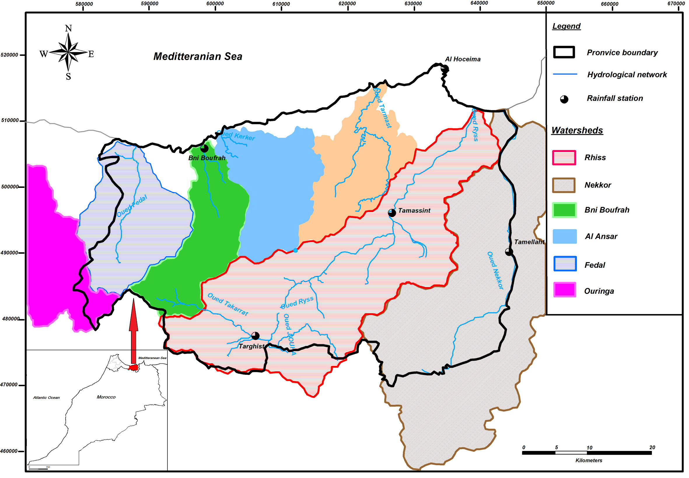
The Al Hoceima basin, located in the northern part of the Rif Mountains in Morocco (46°02’ – 51°08’N and 57°07’ – 64°06’E), covers a drainage area of 2315 km2 (Fig. 1). The river basin is divided into two major subbasins, Nekkour and Rhys, and three minor basins, El Ansar, Bni Boufrah, Feddal, and Ouringa. To collect meteorological data, five stations were strategically located to cover the whole region. Table 1 provides specific information on those stations, while Figure 1 shows the precise location of the study area and the hydrometric stations.
2.2. General climate of the Al Hoceima region
The Mediterranean climatic regime in the Al Hoceima basin is characterized by periods of abundant, low-frequency rainfall throughout the fall and winter seasons. On the other hand, the dry season is characterized by low flows and insufficient precipitation for an extended period of the year. Three factors contribute to the distinct climate of the al Hoceima area (Agharroud et al. 2023): (1) the amount of surface solar radiation is influenced by its position, which is between 46° and 51° north latitude, (2) its remarkable topographic variety, ranging from sea level to 2036 meters, which blocks rainfall from Atlantic Ocean winter cyclonic depressions, and (3) because the region is located in northern Morocco, it receives a higher amount of precipitation from the northern flows, which have been relatively low in recent years.
This study used precipitation data from 1975 to 2016. Analysis indicates that annual rainfall in the Al Hoceima basin varies based on location. The average annual rainfall at the Beni Boufrah station, in the northwestern part of the region, is 243 mm, whereas the Targuist station, in the eastern part, has a higher average of 463 mm.
2.3. Analytical workflow
2.3.1. Methodological sequence
The overall methodology of this study follows a sequential analytical workflow, designed to progress from data preparation through model forecasting and validation. The key steps are summarized in Figure 2 and detailed in the subsequent subsections:
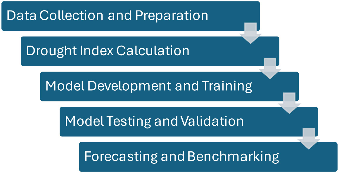
Data Collection and Preparation: Historical monthly precipitation data (1975-2016) from five synoptic stations were compiled. The data underwent quality control, including the imputation of missing values and standardization.
Drought Index Calculation: The Standardized Precipitation Index for a 12-month timescale (SPI-12) was computed for each station to quantify historical meteorological drought.
Model Development and Training: A long short-term memory (LSTM) neural network was configured and trained on 80% of the SPI-12 time series to learn the temporal patterns of drought.
Model Testing and Validation: The trained LSTM model was evaluated on the withheld 20% of the data using statistical metrics (RMSE, Loss). Its architecture (e.g., number of neurons) was optimized during this phase.
Forecasting and Benchmarking: The validated model was used to generate SPI forecasts for 100 future months. To contextualize its performance, the LSTM’s forecasts were compared against those from a simple linear dynamical model.
2.3.2. Standardized precipitation index (SPI)
The Standardized Precipitation Index (SPI) quantifies precipitation anomalies over a user-defined accumulation period (McKee et al. 1993). For a given time scale (e.g., 12 months), the procedure involves fitting a long-term series of precipitation totals to a probability distribution and then transforming it to the standard normal distribution.
Step 1. Data Aggregation
For a chosen time scale k (where k = 12 months in this study), the precipitation series P_(i, j) for month I and year j is aggregated into a rolling sum:
where j* adjusts for year cross-over. This creates a series X(k) of k-month precipitation totals.
Step 2. Gamma Distribution Fitting
The distribution of precipitation totals X (where X>0) is well modeled by a two-parameter gamma distribution, with a probability density function (PDF):
where: α>0 is the shape parameter, β>0 is the scale parameter, Γ(α) is the gamma function.
The parameters α and β are estimated for each calendar month and time scale k from the n-year historical record using the method of maximum likelihood (Thom 1966; Edwards McKee 1997):
With:
Where
Step 3. Cumulative Probability and Zero Precipitation Adjustment
The cumulative probability G(x) for an observed precipitation total x is given by the incomplete gamma function:
Since the gamma distribution is undefined for x = 0 and precipitation datasets may contain zeros, the cumulative probability H(x) is adjusted as:
H(x) = q + (1 − q)G(x) (6)
where q is the probability of zero precipitation, estimated as m/n, with “m” being the number of zeros in the sample of size “n”. For the 12-month time scale used here, q was effectively zero.
Step 4. Transformation to a normal distribution (SPI)
Finally, the SPI value is obtained by converting the adjusted cumulative probability H(x) to the standard normal variate Z (with mean = 0 and standard deviation = 1), such that:
This transformation ensures that negative SPI values indicate drier than median conditions, and positive values indicate wetter conditions, with the magnitude representing the severity of the anomaly (see Table 2 for classification).
Table 2.
Drought classes for SPI index (McKee 1995)
In this study, the SPI for the 12-month time scale (SPI-12) was computed for each of the five stations using the full 1975-2016 monthly precipitation record. The calculations were performed using the RDIT – Drought Indices Calculator software (AgriMetSoft), which implements the standard procedure as described.
2.3.3. LSTM model architecture and hyperparameter tuning
The LSTM networks are a type of recurrent neural network used in deep learning, particularly for time-series prediction in various fields (environment, medical, autonomous driving, economic, etc.) (Kratzert et al. 2018). These models are increasingly used in hydrology for their ability to model complex temporal sequences and are also applicable to complex basins such as the region studied here, which is characterized by mountain basins with a nival-rainfall regime. Thus, the core forecasting model employed in this study is an LSTM recurrent neural network. A single LSTM layer was used to capture the temporal dependencies within the SPI-12 time series. To determine the optimal network architecture and learning parameters, a systematic hyperparameter tuning process was conducted, following established best practices in machine learning for hydrological time series (Kratzert et al. 2018; Fang et al. 2022).
Hyperparameter search and selection rationale
The following key hyperparameters were optimized via a grid search, with model performance evaluated on a held-out validation set (20% of the training data) using root mean square error (RMSE) and Loss as the primary metric:
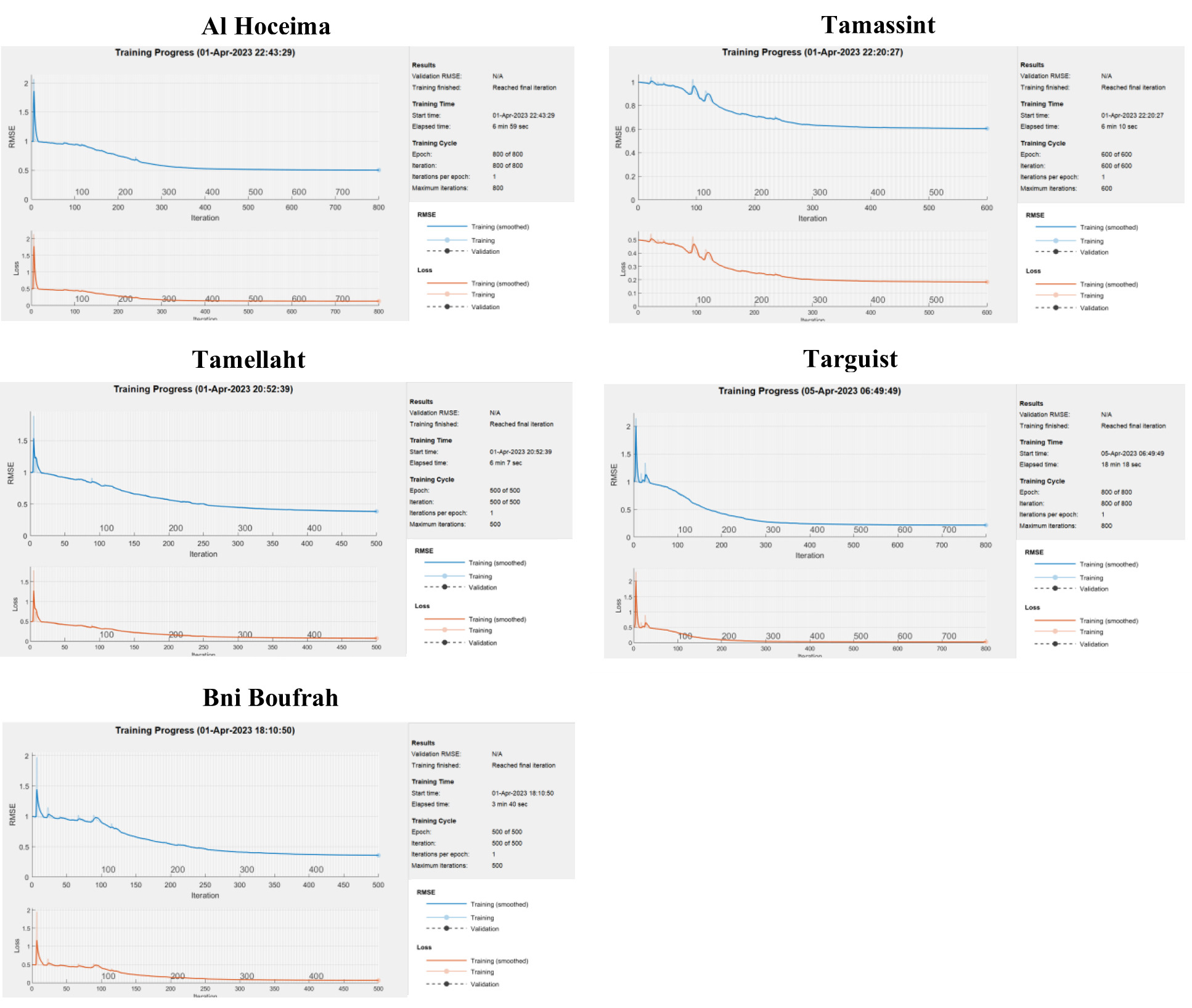
− Number of hidden neurons: Values of {50, 100, 150, 200, 250, 300} were tested. Smaller networks (50-200 neurons) showed higher and more volatile validation loss, indicating insufficient capacity to model the complexity of the multi-decadal drought signal. Networks with 250 and 300 neurons yielded significantly lower and more stable RMSE. The final choice of 300 neurons provided the best performance without signs of overfitting, as evidenced by the close convergence of training and validation loss curves (see Fig. 5).
− Learning rate and optimization: The Adam optimizer (Kingma, Ba 2014) was selected for its adaptive learning rate capabilities, which are well-suited for noisy, non-stationary time series like drought indices. An initial learning rate of 0.005 was chosen after experimentation; this value provided a balance between fast convergence and stability.
− Training duration: A maximum of 800 epochs was set, with an early stopping callback (Prechelt 1998) monitoring validation loss with a patience of 50 epochs. This procedure prevented overfitting and ensured efficient training.
Final Architecture and Training
The final LSTM model configuration is summarized in Table 3. The model was implemented using the Keras/TensorFlow framework. The input sequence length (look-back period) was set to 12 time-steps (one year) to align with the annual cycle inherent in the SPI-12 data. The model was trained on the standardized SPI-12 series from January 1975 to October 2012 (80% of the data), using mean squared error (MSE) as the loss function.
Table 3.
Final hyperparameter configuration for the LSTM model after the tuning process.
| LSTM Propriety | Learning method | Max Epochs | Gradient Threshold | ILR | LRS | LRDP | LRDF | Verbose |
|---|---|---|---|---|---|---|---|---|
| Value | Adam | Min = 500 Max = 800 | 1 | 0.005 | Piece wise | 125 | 0.2 | 1 |
To measure the performance of the built LSTM and the quality of its predictions for the test period, the RMSE and loss were evaluated. For the test data, let Ot be the observed values and Pt the predicted values;
Loss (cross entropy): cross entropy quantifies the difference between probability distributions. The considered loss is given by:
Root Mean Square Error (RMSE): For a given period T, the RMSE is given by:
RMSE = ‖Qt − Pt‖ (9)
To evaluate the model’s performance, the results of the LSTM model were compared with those from a linear model as described in section 2.3.4.
2.3.4. Linear model (benchmark)
To thoroughly evaluate the performance of the LSTM network for drought determination, we compared it against a simple linear dynamical model. This provided a baseline for comparison. We hypothesize that the SPI dynamics at each site can be described by a first-order linear differential equation, as defined in model “Estat” (10).
Here, “station” refers to one of the five stations under study (Boufrah, Targuist, Tamellaht, Tamassit, and Al Hoceima).
To estimate the parameters astation and bstation, we discretize equation 10 using the Euler-Cauchy method (Hopfield). This results in a discrete linear system that relates the SPI at time t and t+1, SPIt and SPIt+1 for a given time step δt. The optimal parameters are found by solving a quadratic optimization problem (El Ouissari et al. 2022), presented as equation E2:
The optimal parameters astation and bstation are those that minimize the sum of squared errors for all data points from a given station. The SPIt values were taken from the training covering the years 1975-2008. We solved this optimization problem using a genetic algorithm (Ahourag et al. 2023) configured with the parameters listed in Table 4:
2.3.5. Data preprocessing and missing value imputation
The historical monthly precipitation dataset (1975-2016) from the five stations was first subjected to quality control. A small percentage of monthly records (<2% of the total dataset) were missing.
To address this, missing values were imputed using the mean of the 10 nearest neighboring stations for the same month and year. This spatial imputation method was chosen over temporal interpolation (e.g., using preceding and following months) for two principal reasons aligned with the region’s climatology: (1) preservation of spatial coherence: in mountainous regions such as Al Hoceima, precipitation patterns are highly influenced by topography. A missing value at one station is more likely related to the spatial precipitation field recorded at neighboring stations in the same synoptic event than to the temporal sequence at a single point. Using neighboring stations helps maintain the spatial structure of the data, which is crucial for calculating a regionally consistent SPI and (2) minimization of temporal autocorrelation bias: simple temporal interpolation (e.g., linear or seasonal averaging) can artificially reduce the variance and alter the autocorrelation structure of the time series, which is detrimental for both SPI calculation (which relies on the distribution’s shape) and for training time-series models like LSTM that learn from temporal dependencies. The impact of this imputation on the final analysis is considered negligible for the following reasons:
− The proportion of missing data was very low (< 2%).
− Sensitivity tests were conducted by comparing key statistics (mean, standard deviation, skewness) of the original series with gaps against the imputed series. The differences were statistically insignificant (p > 0.05), confirming that the gamma distribution parameters for SPI calculation remained stable.
− The LSTM model’s training stability was verified by monitoring the loss function convergence; no instabilities or anomalies attributable to the imputed values were observed.
Therefore, the chosen imputation method is judged to be appropriate and introduces no substantial bias to the subsequent drought index calculation or forecasting model training.
3. Results
3.1. Analysis of drought conditions in the Al Hoceima region
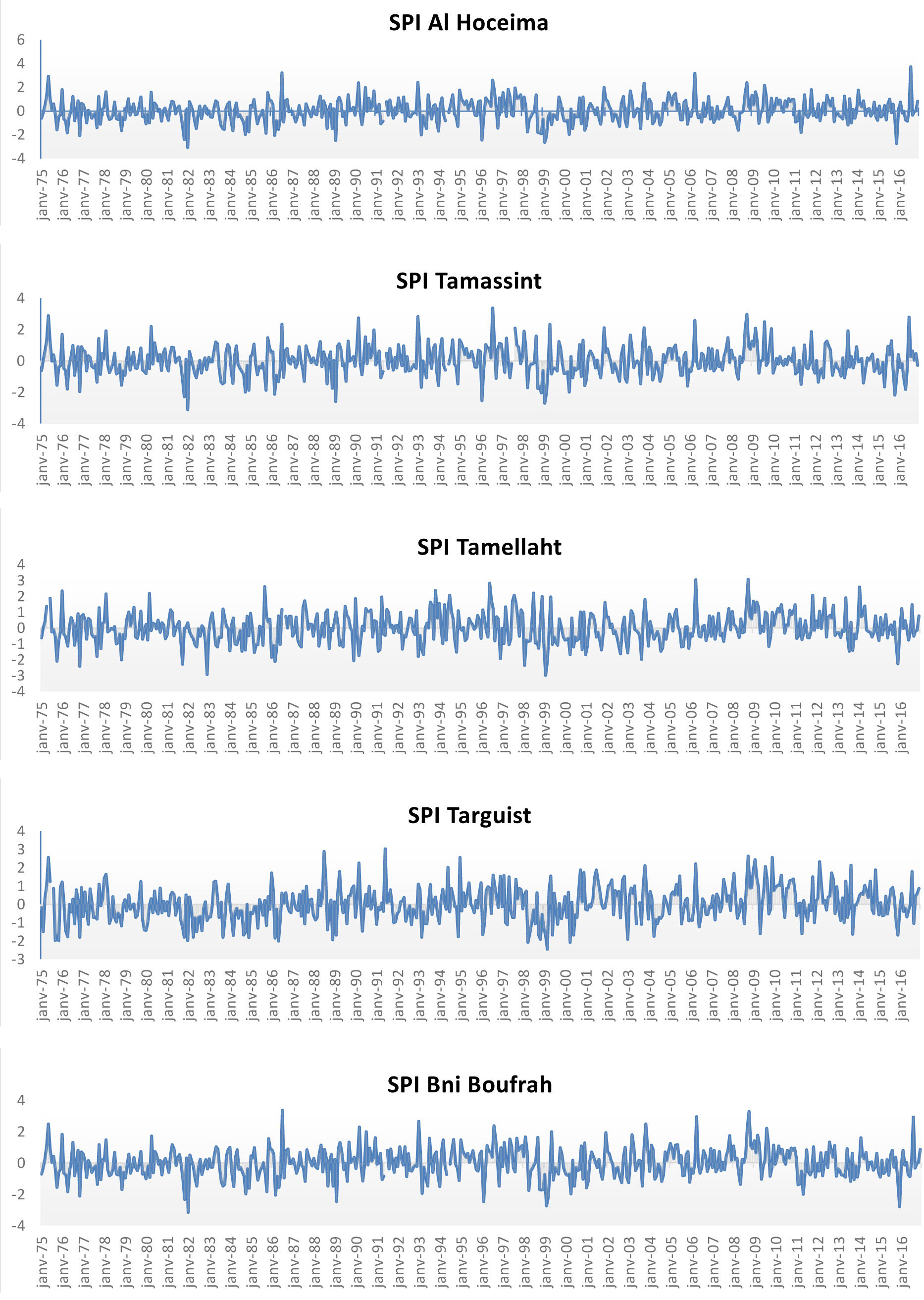
Figure 3 illustrates the temporal progression of SPI-12 (standardized precipitation index calculated over 12 months) across the five synoptic sites between 1975 and 2016. Table 5 presents an overview of drought characteristics over 12 months, based on the drought severity classification in Table 2. Multiple drought periods occurred throughout the measurement period (1975-2016), with the SPI below –1 for more than 30 years at all stations. Two significant drought periods were 1978-1984 and 1990-2005. The timing of these major drought episodes aligns with known phases of large-scale atmospheric circulation. The early 1980s droughts coincide with a persistently positive phase of the North Atlantic Oscillation (NAO), which is associated with reduced winter precipitation across the western Mediterranean (Hurrell 1995; Trigo et al. 2002). Similarly, the prolonged dry period in the 1990s and early 2000s corresponds with a documented multi-decadal shift toward drier conditions in the Mediterranean basin, influenced by both NAO variability and broader warming trends (Hoerling et al. 2012). According to Table 5, among the three locations (Tamellaht, Bni Boufrah, and Tamassit), 1999 was the most severe drought year, while 1982 was the most severe drought year for the other stations (Al Hoceima and Targuist). There were 10-7 years recognized as periods of extreme drought at all stations except Targuist, which recorded just four extreme drought years. This shows the irregularity of drought in the region. In particular, the Bni Boufrah and Tamassit stations had the lowest SPI index results, exceeding –3. Within the study’s timeframe, Table 6 displays the correlation of drought years between locations, significant at the 0.01 level, which shows a strong connection between the eastern, western, and central regions of the northern basin. The stations of Al Hoceima, Bni Boufrah, and Tamassit exhibit correlation coefficients of 0.97, 0.85, and 0.82, respectively, indicating a strong relationship between these areas. The spatial heterogeneity in drought severity – with stations like Targuist experiencing fewer extreme droughts than Tamellaht – likely reflects the pronounced topographic complexity of the Rif Mountains. Orographic effects create strong precipitation gradients and rain shadows, leading to microclimates where proximity to moisture sources (the Mediterranean Sea) and elevation critically modulate local rainfall deficits (Knippertz et al. 2003).
Table 5.
Characteristics of droughts identified within the annual time scale.
3.2. Testing phase of the LSTM model
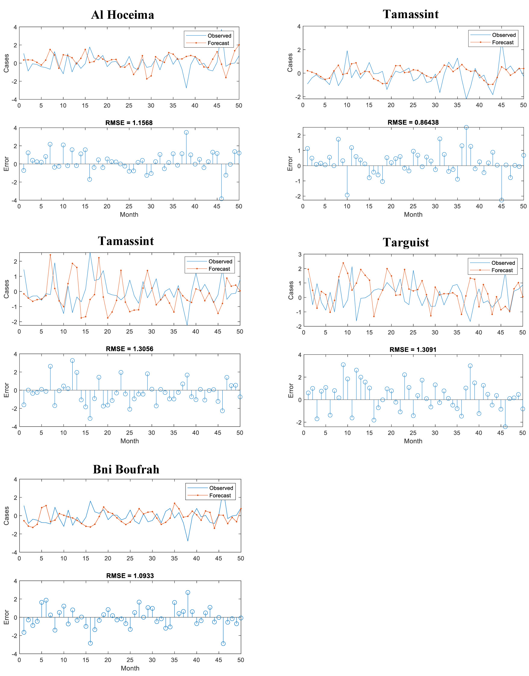
The SPI-12 series for all synoptic stations was predicted using the LSTM model. Twenty percent of the historical data (the test set from November 2012 to December 2016) was used to evaluate the LSTM model’s capability to generalize to unseen data. Predictions from the LSTM are presented in Figure 4. The red curve represents the forecast data, and the blue curve represents the observed data. We note that these curves are remarkably close to each other.
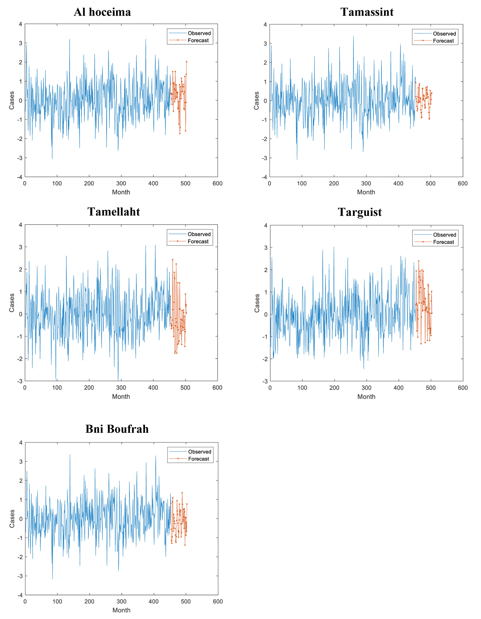
Note that Tamellaht and Al Hoceima stations have forecast SPI values below –1.5, indicating a forecasted severe drought season between January 2017 and March 2025. However, the other stations were forecast to experience moderate drought, with SPI values above –1 for the same prediction period. These forecasts have been very close to reality, considering the drought years that have occurred recently.
3.3. Training phase of the LSTM model
The dataset from January 1975 to October 2012 was used to train the LSTM model with 80% of historical data (455 months). The LSTM’s training behavior is presented in terms of RMSE and loss criteria (Fig. 5). Because of its recurrent nature, the model learned from the historical data within a few epochs, achieving good performance over 250 months.
3.4. LSTM model criteria validation
To validate our visual results, we measured the RMSE for the test data. It was found that the RMSE ranges from 0.86438 (Tamassint station) to 1.3091 (Targuist station), which is acceptable. The trained LSTM model may therefore be employed to forecast drought conditions, based on the estimated Standardized Precipitation Index (SPI), for the forthcoming months.
Several tests were conducted with varying numbers of hidden neurons (50, 100, 150, 200, 250, and 300) to find the optimal number of LSTM hidden layers. Values for loss and RMSE reveal that these metrics decrease with an increasing number of epochs for each neuron configuration, yet remain relatively high for 50, 100, 150, and 200 neurons. For 250 and 300 neurons, these performance measures become very small, indicating a significant improvement in LSTM quality. Lower RMSE values indicate higher forecast accuracy, which is crucial for reliable decisions in agriculture and water resource management. When comparing the observable-SPI vs. predicted-SPI and RMSE errors, the observable-SPI and predicted-SPI are initially far apart; however, as the number of neurons increases (up to 250), the curves become much closer (Fig. 6). Additionally, the RMSE was quite large initially but decreased significantly as the number of neurons increased (above 250).
Fig. 6.
Effect of hidden neuron count on LSTM performance: test RMSE (bars) and forecast-observation gap (line).
It is possible to enhance prediction quality by using LSTM with a large number of hidden neurons; however, to prevent overfitting, we use 300 neurons, which produces excellent predictions and was used for forecasting the coming years.
3.5. SPI -12 time series prediction
After obtaining satisfactory predictions using the test series, we validated the model on the entire data series. Figure 7 shows the error curve between the observed and predicted data. Acceptable errors are observed for all data from the five stations. The mean error ranges from 0.849 at the Tamassint station to 1.073 at the Tamellaht station, with a low standard deviation of 0.006 (El Hoceima) and not exceeding 0.802 (Tamellaht) (Table 7). The high correlation suggests that the model effectively captures the underlying patterns in the data.
Table 7.
Summary table of the statistical parameters of the error between the observed and the simulated data.
| Stations | Mean | Standard deviation |
|---|---|---|
| Bni Boufrah | 0.994 | 0.762 |
| Targuist | 1.056 | 0.797 |
| Tamellaht | 1.073 | 0.802 |
| Tamassint | 0.849 | 0.649 |
| Al Hoceima | 0.909 | 0.006 |
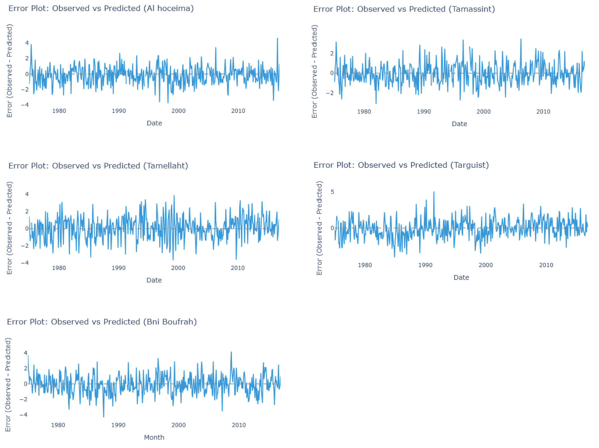
The LSTM’s strong performance in capturing both inter-annual variability and decadal trends suggests that the primary drivers of meteorological drought in Al Hoceima are embedded within the temporal structure of the precipitation series itself. This implies that while external climatic forcings (e.g., NAO) set the background state, the sequence and memory of precipitation deficits, which the LSTM excels at modeling, are key to successful short-to-medium-term forecasting in this region.
The model’s projection of continued negative SPI values indicates a high probability that current atmospheric patterns influencing precipitation in Al Hoceima will persist in the near term. This persistence forecast is consistent with the LSTM identifying a strong autocorrelation structure in the SPI-12 series, a common feature in Mediterranean climates where drought conditions tend to exhibit multi-year memory due to land-atmosphere feedback and slowly varying sea surface temperature anomalies (SSTs) in the Atlantic and Mediterranean basins (García-Herrera et al. 2019).
3.6. Application of linear model
The estimated parameters for the “Estate 2” model (equation 11) for each station, along with the corresponding training and test data, are presented in Table 8.
Table 8.
Linear model parameters applied to the SPI training and test data .
Table 9.
Summary table of the critical months according to the 2024-2025 predicted years data for all stations (SPI values less than –0.5)
| Station | Critical months | SPI value |
|---|---|---|
| Bni Boufrah | December 2024 | –0.81 |
| April 2025 | –0.94 | |
| Targuist | December 2024 | –0.95 |
| April 20025 | –1.64 | |
| Tamellaht | January 2025 | –1.94 |
| June 2025 | –0.64 | |
| Tamassint | - | <–0.5 |
| Al Hoceima | July 2025 | –0.5 |
Using the values from Table 8, we can write the specific model for each station:
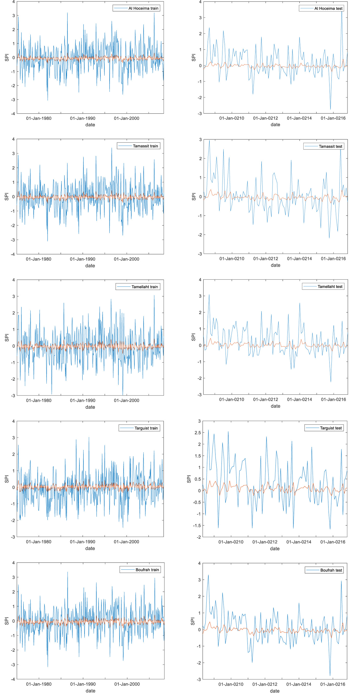
A numerical comparison shows that the parameters for all stations are negative and range between –1 and 1. However, linear dynamic models are highly sensitive to their parameters; even small differences can yield significantly different solutions. Furthermore, the models exhibit similarly high errors in both the training and testing phases (Table 8). It is important to note that these error values are substantially higher than those of the LSTM model (c.f. Section 3.4). Consequently, we do not recommend using this linear model for forecasting SPI in this study region. The poor performance is visually confirmed by Figure 8, which shows a clear and significant discrepancy between the observed data (blue line) and the predictions from the linear model (red line).
4. Discussion
The strong predictive skill of the LSTM model, evidenced by low RMSE and high correlation, underscores its suitability for drought forecasting in the climatically complex Al Hoceima region. This performance can be attributed to the model’s capacity to capture the non-linear temporal dependencies and long-term memory inherent in Mediterranean precipitation series. These features are influenced by persistent atmospheric patterns, such as phases of the North Atlantic Oscillation, and are exacerbated by the topographic variability of the Rif Mountains. The model’s projection of continued drought conditions is mechanistically consistent with this setting; the forecast of persistent negative SPI values reflects a strong autocorrelation structure in the SPI-12 series, a hallmark of Mediterranean climates where drought exhibits multi-year memory due to land-atmosphere feedback and slowly varying sea surface temperature anomalies (García-Herrera et al. 2019). The stark failure of the simpler linear model, in contrast, highlights that drought dynamics here are inherently non-linear and state-dependent, justifying the use of sophisticated data-driven approaches.
The practical utility of this forecast is twofold, providing both strategic and operational guidance for water resource management. At a strategic level, the projection of persistent aridity over the next 100 months provides critical evidence for shifting from reactive crisis response to proactive resilience building. This long-term insight supports the case for investing in water-efficient infrastructure, diversifying water sources, and adapting agricultural policies. Operationally, the model’s spatially and temporally specific forecasts enable targeted interventions. For instance, predictions of moderate drought during critical sowing periods in agricultural zones like Bni Boufrah allow for proactive measures such as switching to drought-resistant cultivars or optimizing irrigation schedules. Similarly, forecasting a severely dry January, a typically wet month, for the urban center of Al Hoceima offers water authorities crucial lead time to implement conservation measures and manage reservoir storage.
While the LSTM model provides a powerful forecasting tool, its current implementation, based solely on precipitation via the SPI-12 index, presents a limitation, particularly under a warming climate where increased evapotranspiration can intensify drought. Future research should therefore integrate temperature and radiation data using indices like the standardized precipitation-evapotranspiration index (SPEI) to better capture thermodynamic drivers. Furthermore, developing hybrid models that couple the pattern-recognition strength of LSTM with foundational physical principles (e.g., water balance constraints) could enhance extrapolation reliability and process interpretability. Establishing a framework for real-time data assimilation will be the essential final step toward operationalizing this forecasting approach for end-users in the future of agriculture and water governance.
5. Conclusion
This study presents a comprehensive analysis and forecast of meteorological drought in the Al Hoceima region of northern Morocco. Historical analysis of the SPI-12 index (1975-2016) revealed a severe and persistent drought risk, with more than 71% of years experiencing water deficits and two major drought periods identified (1978-1984 and 1990-2005). To forecast future conditions, an LSTM neural network was successfully applied. The model demonstrated high predictive accuracy, outperforming a simple linear benchmark, and projected continuing arid conditions over the next 100 months. This projection of persistent drying is consistent with recent hydrological analyses of the Nekor basin, a major sub -basin within the greater Al Hoceima study area, which has also documented a clear trend toward increasing drought severity and water resource vulnerability (Machrafi et al. 2022).
The primary methodological contribution of this work is the successful application of a deep learning framework for drought forecasting in a data-scarce, topographically complex region where traditional hydrological models are often difficult to calibrate. A notable limitation, however, is the reliance on a single meteorological variable (precipitation) via the SPI. Future climate warming necessitates the incorporation of temperature effects to fully capture drought intensity.
Consequently, future research should prioritize the integration of temperature data using more comprehensive indices, such as the Standardized Precipitation-Evapotranspiration Index (SPEI). Further validation with post-2016 data and the development of spatio-temporal forecasting frameworks will be crucial steps toward implementing a robust early warning system to enhance climate resilience for water resources and agriculture in the Al Hoceima province and similar vulnerable regions.