1. Introduction
Water is a key aspect for economic development, including agricultural and industrial expansion, particularly in the context of rapidly growing population and urbanization. Under changing land use and climate, sustainable water resource management and optimal allocation of water resources across multiple water uses are key difficulties that many civilizations are either facing or will confront in the next decades (Stehr et al. 2008). To address water management challenges, we must investigate and evaluate the many aspects of hydrologic processes occurring within the study area. Because all of these activities occur within separate micro-watersheds, the studies must be done on a watershed basis. For understanding the complicated hydrological response of a watershed and its direct relationship to climate, geography, geology, and land use, advanced mathematical models have been constructed. Water flows not just over the surface of land, but also underneath it in the unsaturated zone and even deeper in the saturated zone (Singh, Woolhiser 2002). Simulating these processes through a watershed model is essential for addressing a variety of water resource, environmental, and social issues. SWAT model predictions have been deemed computationally efficient by researchers (Neitsch et al. 2005). The tool has shown dependability in numerous regions throughout the world. Khan et al. (2014) used the SWAT model on a large scale to examine hydrological processes in a mountainous environment of the Upper Indus River Basin, as well as in other Asian locations (Supit, Ohgushi 2012; Nasrin et al. 2013).
Beroho et al. (2025) investigated the 9th April watershed in northern Morocco, a semi-arid region with limited hydrometeorological data. They integrated SWAT with projected land use-land cover (LULC) and climate scenarios to model future hydrological responses and sediment transport. Fadil et al. (2011) employed it in several African locations. Schuol et al. (2008) and Ashagre (2009) also used it in simulations. Kamuju (2019) studied the St. Joseph River watershed in the United States. SWAT is a GIS-based watershed- or river basin-scale model that can represent both geographic diversity and physical processes within smaller modeling units known as hydrologic response units (HRUs) for the long -term planning and management of river surface water resources. Its predictions have been declared computationally effective by researchers (Neitsch et al. 2009). It has been proven to be reliable in a majority of places globally.
2. Materials and methods
2.1 Study area
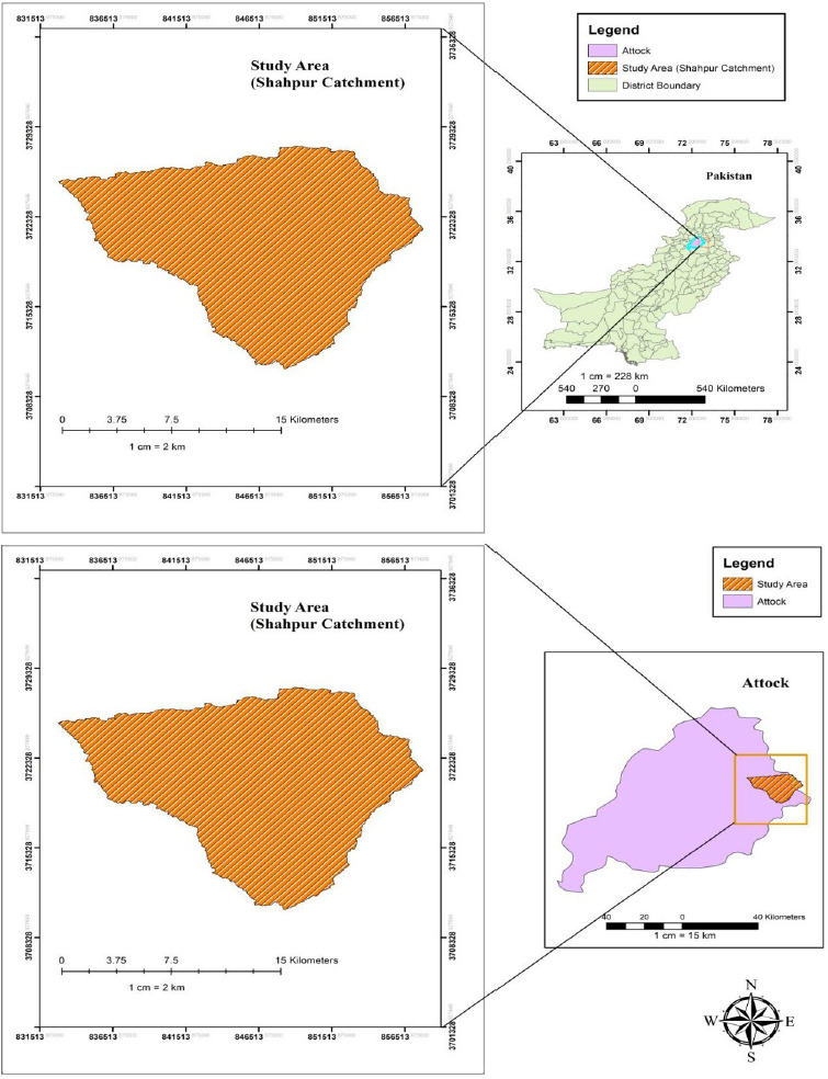
We selected the Shahpur Dam as a study site to perform hydrological modeling by using SWAT and GIS analysis. The dam site is located at 33°37'0'', 73°41'0''E in Fateh Jang Tehsil near the Kala Chitta Range in the Attock District, about 45 km from Islamabad and 8 km north of Fateh Jang, as shown in Figure 1. The dam was commissioned by the Small Dams Organization, Government of Punjab, in 1982 and was completed in 1986 at a cost of PKR 36.5 million. The main dam is a concrete gravity type with 0.6 m thick stone masonry skin and a centrally located spillway. There is an ungated ogee spillway in the middle of the dam for passing flood discharges. The capacity of the spillway is 1008 m3/s. This discharge is based on 230 mm rainfall, which is the maximum probable in 24 hours with a 1000-year return period. The width of the spillway is 85 m, which could easily handle a discharge of 460 m3/sec with a head of 3 m above the crest. A flip-type stilling basin was installed to dissipate the energy of falling water from the spillway. The reservoir of Shahpur Dam has a gross storage capacity of 14,320 acre-feet (17.7×10⁶m3), of which 4,079 acre-feet (5.0×10⁶m3) is dead storage capacity and the rest is live usable storage (Cheema, Bandaragoda 1997; Ghumman et al. 2019).
2.2. Creation of database
2.2.1 Time-based datasets
SWAT requires climate data to supply moisture and energy inputs that govern the water balance and establish the key results of the various components of the hydrological cycle. Hydrological modeling requires long-term meteorological datasets of precipitation, temperature, wind speed, solar radiation, and relative humidity. The minimal essential inputs for the SWAT model are precipitation and temperature, whereas the remaining factors are optional. The model’s weather-generating feature allows it to create data based on these inputs (Ghoraba 2015). Weather data (daily maximum and minimum temperature, relative humidity, and wind speed) of the study area is obtained from PMD Islamabad.
The Shahpur Dam site office, located in Fateh Jhang, provided daily precipitation data. Historic daily flow data were provided for the years 2000-2004 for calibration and 2006-2010 for flow simulation validation. The monthly inflow to Shahpur Dam was measured at a station located near the dam.
2.2.2. Spatial datasets
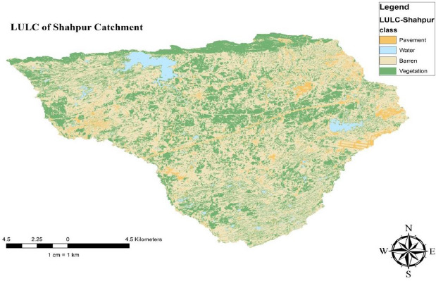
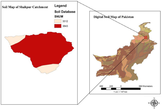
Topography, land use-land cover, and soil composition are spatial datasets that characterize every land system and are essential for the hydrological model (Arnold et al. 1998). The input element of the SWAT model involves components of the land system that consist of DEM, land use, and soil (Ghoraba 2015). The DEM is downloaded from the Earth Explorer of the United States Geological Survey (USGS). Then, using the extract-by-mask feature, the study region is isolated from the large DEM file shown in Figure 2. For delineation, an SRTM DEM with resolution 30 m × 30 m was used. The automatic watershed delineation feature was applied to define the watershed. Landsat 8 satellite imagery was used to create a land use map through supervised classification, employing ERDAS IMAGINE 2012, as shown in Figure 3 (Beroho et al. 2023). The water cycle is affected by changes in land use and vegetation; the impact depends on the species’ morphology and plant cover density. Four main classes have been defined. The most important groups are urban (4.84%), water (2.71%), barren (57.63%), and agricultural land (34.82%). The original land use classes were replaced with SWAT classes and specified using a lookup table. These conversions are presented in Table 1. For this research, two types of soil shown in Table 1 were found in SWAT by using a soil map, which was downloaded from FAO maps. The study area was clipped by the clip feature in Arc GIS, also shown in Figure 4 (Malik et al. 2022).
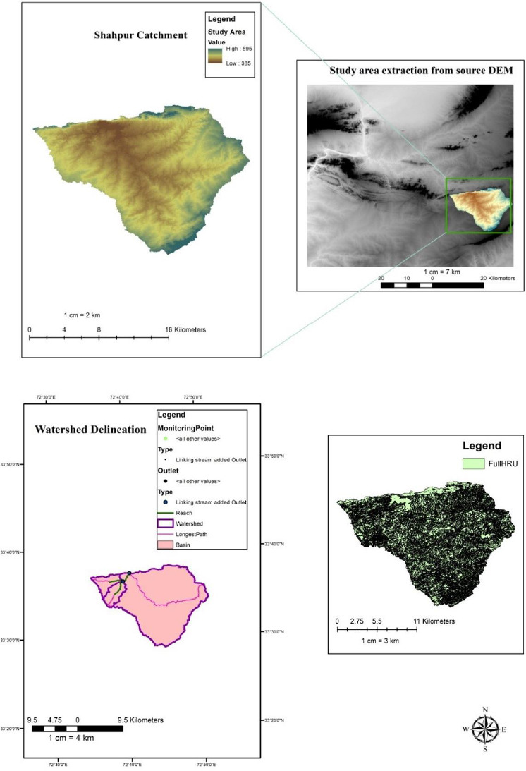
Fig. 3.
Land use-land cover of Shahpur Catchment. LULC Mapping: LULC classes were mapped to SWAT land cover and soil classes using standard lookup tables, derived from FAO soil maps and Landsat 8 imagery, ensuring accurate representation of the catchment’s spatial characteristics.
2.3. Model simulation
The Shahpur Dam watershed hydrologic modeling was performed using Arc SWAT 2012 version 10.5.24, which was created for Arc Map 10.5. The model is ready for simulation once data files have been prepared, and all model inputs have been finalized. The simulation spans four years, from 2000 to 2004, which coincides with the availability of climatic data.
2.4. Model efficiency
Model calibration and validation are important steps in the simulation, applied to evaluate parameter estimation outcomes. There are several approaches for assessing and evaluating the model’s efficiency. The coefficient of determination (R2), root-mean-square error (RMSE), standard deviation ratio (RSR), Nash–Sutcliffe efficiency index (NSE), and percent bias (PBIAS) were used for calibration and validation (Moriasi et al. 2007; Fadil et al. 2011).
2.4.1. Coefficient of determination (R2)
By following a best fit line, it is an excellent approach to indicate the consistency between observed and simulated data. Higher values indicate less error variance, and values greater than 0.50 are regarded as acceptable. It ranges from zero to 1.0 (Santhi et al. 2001; Van Liew et al. 2007).
Where Qs,j is the discharge flow’s simulated value, Qm,j is the discharge flow’s measured value, and Qm is the mean of the measured discharge flow; n is the length of the measured discharge, and Qs is the mean of the simulated discharge flow.
2.4.2. Nash–Sutcliffe efficiency (NSE )
NSE is a normalized statistical approach for predicting the relative level of noise vs data.
Where Ysimi is the ith simulation, and Yobsi is the ith observation (stream flow), the mean of the actual data, Ymeani is the simulated value, and n is the sum of all observations (Nash, Sutcliffe 1970).
2.4.3. Percent bias (PBIAS)
PBIAS calculates the average tendency of simulated values to be greater or lower than observed values. The statistic ranges from –10 to +10. PBIAS has an optimum value of 0.0, with low-magnitude values indicating accurate model simulation. Positive values indicate model underestimation bias, whereas negative values suggest model overestimation bias (Gupta et al. 1999).
2.4.4. RMSE-RSR
An RSR range of 0 to 0.5 indicates good performance for both the calibration and validation periods. The lower the value of RSR, the smaller the RMSE as normalized by the standard deviation of the data, indicating the precision of the model simulation (Singh et al. 2005).
3. Results
3.1. Parameter sensitivity analysis
After running the SWAT model, the model parameters must be calibrated and analyzed for sensitivity. Based on a literature review, 11 factors with stronger influence on runoff were chosen, supported by Arnold et al. (2012) and Abbaspour (2007). The (SUFI2) algorithm was used to determine the parameters in this project. To achieve the best match between the model’s output and the observed flow data, the model is repeatedly simulated by adjusting the evapotranspiration calculation technique and the values of hydrological parameters that were selected by the model.
3.2. Model calibration and validation results
The SWAT-CUP tool is one of the best tools for calibrating the SWAT model, and it is appropriate for assisting decision-makers in conceptualizing sustainable watershed management, allowing decision-makers to better calibrate the model (Mengistu et al. 2019). The simulated and actual surface runoff were compared for calibration. Only the fundamental scale and range of values generated by the model were verified using monitoring data. The exact value of calibrated hydrological parameters was utilized for validation after obtaining acceptable runoff data. Following that, the model’s performance with calibrated parameters was evaluated to recreate the hydrological functioning of the watershed over a period that was not employed in the calibration phase. The observed flow data obtained from the Shahpur Dam site office, recorded at a gauging station downstream from the Shahpur Dam on the Nandana River, were used for flow calibration and validation. The available data were compared to the projected results to determine the effectiveness of the SWAT simulation. The calibration was performed on a monthly and an annual basis using outflow data from 2000 to 2004; the parameters were then validated between 2006 and 2010. To reduce the gap between the simulated and actual values, 11 model parameters (Table 2) were adjusted (Arnold et al. 2012).
Table 2.
Parameter descriptions.
All sub-watersheds received a 2% increase in CN2, a 0.3% increase in ALPHA BF, a 0.1% increase in GW DELAY, a 0.5% increase in GWQMN, a 0.3% increase in SLSUBBSN, a 0.4% increase in SURLAG, a 3% increase in OV N, and a 0.35% increase in ESCO. SOL-AWC and CH N2, the starting parameters, were multiplied by 1.2 and 0.3, respectively (Abbaspour 2007). The calibration of the model for various water balance components produced satisfactory agreement (Gasirabo et al. 2023).
3.3. Graphical comparison of calibration and validation results
Predicted and actual yearly flows over the calibration period are compared in Figure 5. The average flow for the simulated period was 11.89 m3/s, whereas the average actual flow over the same time was about 13.00 m3/s. Maximum flow was in 2003; minimum flow was in 2000. Depending on the meteorological information obtained from the PMD, the simulation results demonstrate a good fit with peak and low-flow periods. According to Figure 6, the flow results for the validation period indicate good agreement between observed and model-simulated data. The simulation’s average annual flow was 24.45 m3/s, whereas the average measured flow over the same period was 26.16 m3/s, a close match. The findings indicate that the model can be successfully applied to forecast annual average river flow levels. The R2 statistics for calibration and validation, indicating the reliability of the findings, are displayed in Figures 7 and 8, where R2 is 0.99 and 0.96, respectively, demonstrating that the model findings for both periods are excellent. The model’s annual stream flow data indicated a PBIAS of 1.8 for the calibration period and 0.51 for the validation period. These numbers show that the model overestimated stream flow during the validation period while simulating stream flow with a less precise model during the calibration phase. RSR was 0.52 for the calibration period and 0.29 for the validation period, according to the data. Table 5 and 6 provide summaries of the statistical analysis of simulated and actual yearly stream flow data. Based on NSE, the model results for calibration (0.91) and for validation (0.86) are both satisfactory. Monthly flow model results are also depicted in Figures 9, 10, 11, and 12 with R2 values that are quite acceptable. The modeled monthly stream flow data indicated a PBIAS of 0.34 for the calibration period and 0.08 for the validation period. These numbers show that the model overestimated stream flow during the validation period while simulating stream flow with a less precise model during the calibration phase. RSR was 0.23 for the calibration period and 0.31 for the validation period, according to the data. Table 3 and 4 provide summaries of the statistical analysis of simulated and actual monthly stream flow data. According to the NSE approach, the model results of 0.89 for calibration and 0.58 for validation are both satisfactory. The simulation underestimates the peak flow values experienced in January, May, and September. The location of the peaks was generally well-simulated for both the calibration and validation periods. If additional precipitation and temperature datasets from meteorological observatories with specific coverage of the research region were available, the model results might be enhanced significantly and achieve outstanding accuracy. Numerous studies have shown the SWAT model’s under-prediction of peak flows (Fadil et al. 2011; Ghoraba 2015).
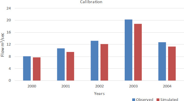
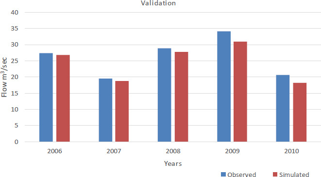
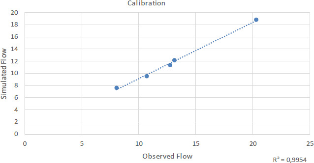
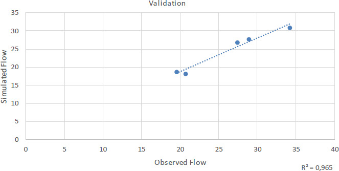
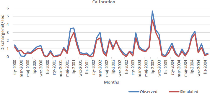
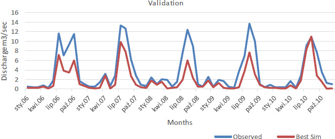
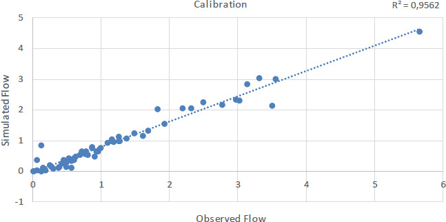
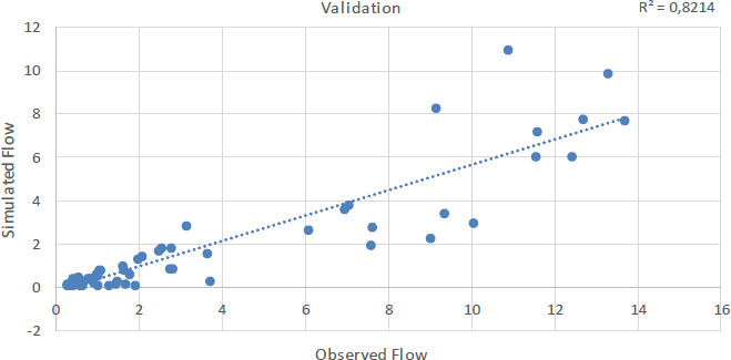
Table 3.
Statistical analysis of simulated and actual monthly stream flow for calibration.
| Calibration (2000-2004) | Observed | Simulated |
|---|---|---|
| Mean | 1.16 | 0.92 |
| R2 | 0.95 | |
| NSE | 0.89 | |
| PBIAS | 0.34 | |
| RSR | 0.23 | |
Table 4.
Statistical analysis of simulated and actual monthly stream flow for validation.
| (2006-2010) | Observed | Simulated |
|---|---|---|
| Mean | 3.58 | 1.90 |
| R2 | 0.82 | |
| NSE | 0.58 | |
| PBIAS | 0.08 | |
| RSR | 0.31 | |
3.4. Water balance components
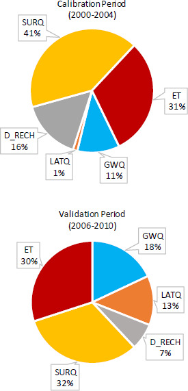
In addition to annual and monthly flow, the SWAT model assessed additional essential water balance components. According to (Sathian, Shyamala 2009), the most essential aspects of a basin’s water balance are precipitation, surface runoff, lateral flow, base flow, and evapotranspiration (Arnold et al. 1998). Except for precipitation, all of these variables require prediction to be quantified because their measurement is difficult. The average annual basin values for various water balance components throughout the model’s simulations of the calibration and validation periods are presented in Table 7, computed as a proportion of the annual rainfall average in Figure 13. Among these aspects, actual evapotranspiration (ET) generated the most water loss from the watershed. A high evapotranspiration rate expected might be ascribed to the type of plant cover and high temperature associated with the location. For the calibration period, the average annual evapotranspiration is 0.31, and for the validation period, the value is 0.30. The quantity of stream flow leaving the watershed’s outflow during the time step is known as total water yield (WYLD). The majority of the rainfall received by the basin is lost as stream flow, as can be observed. On the other hand, for the calibration period, the ratio of the simulated average annual surface runoff to the average annual precipitation is 0.41 and 0.32 for the validation period. The lateral flow (Lat Q) was significantly impacted by the terrain slope. As the slope rises, the lateral flow, calculated as a proportion of annual rainfall average, is 1% for the calibration period and 13% for the validation period. Therefore, lateral flow is a crucial factor in river flow on sloping terrain. It has little effect on shallowly sloped ground. Deep aquifer recharging is substantial in all situations, with average percentages of 16% and 7% of total rainfall for both simulated periods. The water from the shallow aquifer that returns to the reach during the time step is known as groundwater contribution to stream flow (GWQ), and it varies greatly among streams. For both the calibration and validation periods, the average annual contribution of groundwater relative to precipitation is 11% and 18%, respectively.
Table 7.
Average annual water balance components.
4. Conclusion and recommendations
The current study attempted to simulate the influence of climatic change, LULC, soil, and topographic conditions on the Shahpur catchment using Arc SWAT 2012 and the input of long-term meteorological data, satellite data, soil data, and DEM images. The Shahpur catchment’s hydrologic model was calibrated and certified using the SWAT-CUP SUFI-2 program to improve the output so that it matches the reported discharge at the gauging station located near the Shahpur Dam site office (Brighenti et al. 2019). The observed flow data obtained from the Shahpur Dam site office, recorded by a gauging station downstream from the Shahpur Dam on the Nandana River, were used for flow calibration and validation. The SWAT model’s effectiveness and capability were determined by the hydrological study in this research project. The model’s efficiency was assessed using accurate calibration from 2000 to 2004 and validation from 2006 to 2010. The calibrated model can be used to investigate the effects of rising temperatures, land use change, and other management-relevant scenarios on streamflow and soil erosion proactively. To evaluate the effectiveness of the model, R2, Nash-Sutcliffe efficiency (NSE), percent bias (PBIAS) and RMSE factors were evaluated for both annual and monthly flows. On an annual basis, manual calibration was conducted first, followed by automatic calibration. On a monthly basis, the model’s calibration and validation generated satisfactory simulation results.
The validation R2 value for monthly stream flow was 0.82%, while the calibration R2 value was 0.95%, demonstrating the symmetric regression of the model. The NSE, which measures how well the model fit the observed data, was 0.58 for validation and 0.89 for calibration. The PBIAS parameter indicates underestimation, with calibration and validation results of 34 and 8%, respectively. The PBIAS parameter displays the difference between the simulated and observed amounts, with a value of 0 ideal. Positive values indicate underestimation, whereas negative values represent overestimation. The validation RMSE value was 0.31%, while the calibration R2 value was 0.23%, for monthly stream flow. The model’s yearly stream flow data indicated a PBIAS of 1.8 for the calibration period and 0.51 for the validation period. These numbers show that the model underestimated stream flow during the validation period while simulating the stream flow with precision during the validation phase. RSR was 0.52 for the calibration period and 0.29 for the validation period, according to the data. The average flow for the simulated period was 11.89 m3/s, while the average real flow was approximately 13.00 m3/s. The flow reached its peak in 2003, with the lowest flow occurring in 2000. The validation period flow result shows good correlations between observed and model-simulated data. The average yearly flow in the simulation was 24.45 m3/s, while the average observed flow over the same period was roughly 26.16 m3/s, suggesting a striking match. The calibration of the model for various water balance components produced satisfactory agreement. The findings of this research suggest that precise water consumption data are required to produce a more accurate representation of water production and the availability of deep aquifer recharge resources with a reduced uncertainty range. Natural year-to-year variability owing to climate, as well as water abstraction and consumption, is included in the stated uncertainty. These results show that the model can correctly anticipate average annual and monthly stream flow levels. It was concluded from the results that if more reliable precipitation and temperature data sets from climatic observatories with good specific coverage of the research region were available, the model results might be greatly improved, with exceptional precision. The hydrological modeling of the Shahpur catchment using the SWAT model revealed important insights but also highlighted several gaps. Limitations in meteorological data restricted the model’s accuracy, suggesting the need for a more comprehensive dataset that includes additional climatic parameters. Additionally, the study primarily focused on surface water without integrating groundwater interactions. Finally, the absence of climate change scenarios indicates a critical area for future research to support effective water resource management. The SWAT model operates on several assumptions about hydrological processes that may not hold true in all contexts. These assumptions could limit the applicability of the model results to other similar catchments. Future research should prioritize enhanced data collection by establishing more meteorological stations to improve model accuracy and real-time monitoring. Integrating advanced remote sensing technologies would provide timely data on land use and vegetation changes. A comprehensive approach using coupled surface and groundwater models is recommended to better understand the hydrological cycle. Previous studies in hydrological modeling have often focused on general applications of the SWAT model in various regions, but many have lacked comprehensive calibration and validation specific to localized settings like the Shahpur catchment. This research provides a hydrological model tailored for the Shahpur catchment, facilitating improved water resource management in a rapidly urbanizing region. The successful calibration and validation of the SWAT model enhance predictive capabilities for streamflow under varying climatic and land use scenarios. Moreover, the findings underscore the importance of localized data integration, which can inform future watershed management strategies and contribute to sustainable development in water-scarce areas. By addressing specific challenges related to water resource allocation, this study contributes valuable insights for policy-making and environmental planning. We propose that this model be employed for Shahpur watershed management based on its robust performance and comparative outcomes.
Most existing studies focus on large river basins, leaving a contextual and methodological gap in applying and validating SWAT in semi-arid regions with limited historical data. This study addresses these gaps by successful calibration and validation of the SWAT model using available data from 2000-2010 for the Shahpur catchment. The results show strong model performance and highlight the model’s potential for effective watershed management. The study is limited by the unavailability of recent meteorological and discharge data, as well as the exclusion of dynamic land use and climate change scenarios. Despite these limitations, the study contributes significantly by establishing a baseline framework for future hydrological modeling in similar environments. We recommend that future research should incorporate high-resolution, more detailed climate and land use datasets, investigate groundwater–surface water interactions, and apply scenario-based modeling to assess the long-term impacts of climate variability and land use change on watershed hydrology.